cs1120 Problem Set 3:
Limning L-System Fractals
- Bring in to class a stapled turn-in containing your written answers to all the questions by 10:01am Wednesday, 23 September. If you worked with a partner, you and your partner should submit a signle writeup with both of your names and UVA Email Ids on it.
- Use our automatic adjudication service to submit a single Scheme file (a modification of ps3.ss) containing all your code answers. You must define an author list. Each partner must separately submit a copy of your joint file. Do this by 9:55am on Wednesday, 23 September.
- Use our automatic adjudication service to submit a single Scheme file and a single PNG file as your answer to Question 12. You must define an author list. Each partner must separately submit copies of the files. For this problem, partners may submit separate files if they choose. Do this by 9:55am on Wednesday, 23 September.
- Complete the Computer Science Department Diversity Survey by 11:59pm on Wednesday, 23 September. (Removed 21 September: there are some problems with the survey. You are not required to do this.)
- If you are doing the extra credit, email your extra credit Scheme definition file to evans@cs.virginia.edu by by 11:59pm on Wednesday, 23 September.
Collaboration Policy - Read Carefully
For this problem set, you may choose to work with a partner of your choice. You are not required to do so.Before starting to work with a partner, you should go through questions 1 and 2 yourself on paper. When you meet with your partner (if any), check if you made the same predictions. If there are any discrepancies, try to decide which is correct before using DrScheme to evaluate the expressions.
If you have a partner, you and your partner should work together on the rest of the assignment. You should read the whole problem set yourself and think about the questions before beginning to work on them with your partner. Both partners need to understand everything you submit.
Remember to follow the pledge you read and signed at the beginning of the semester. For this assignment, you may consult any outside resources, including books, papers, web sites and people, you wish except for materials from previous cs1120, cs150, and cs200 courses. You may consult an outside person (e.g., another friend who is a CS major but is not in this class) who is not a member of the course staff, but that person cannot type anything in for you and all work must remain your own. That is, you can ask general questions such as "can you explain recursion to me?" or "how do lists work in Scheme?", but outside sources should never give you specific answers to problem set questions. If you use resources other than the class materials, lectures and course staff, explain what you used in your turn-in.
You are strongly encouraged to take advantage of the scheduled help hours and office hours for this course.
Purpose
- Practice programming with recursive definitions and procedures
- Explore the power of rewrite rules
- Write recursive functions that manipulate lists
- Make a cs1120 course logo better than "The Great Lambda Tree of Infinite Knowledge and Ultimate Power"
- ps3.ss — A template for your answers. You should do the problem set by editing this file.
- graphics.ss — Scheme code for drawing curves.
- lsystem.ss — provided incomplete code for producing L-System Fractals
Background
In this problem set, you will explore a method of creating fractals known as the Lindenmayer system (or L-system). Aristid Lindemayer, a theoretical biologist at the University of Utrecht, developed the L-system in 1968 as a mathematical theory of plant development. In the late 1980s, he collaborated with Przemyslaw Prusinkiewicz, a computer scientist at the University of Regina, to explore computational properties of the L-system and developed many of the ideas on which this problem set is based.
The idea behind L-system fractals is that we can describe a curve as a list of lines and turns, and create new curves by rewriting old curves. Everything in an L-system curve is either a forward line (denoted by F), or a right turn (denoted by Ra where a is an angle in degrees clockwise). We can denote left turns by using negative angles.
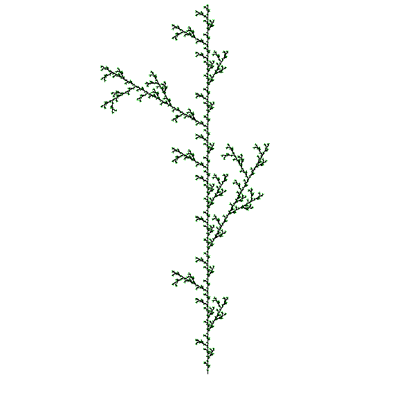
We create fractals by recursively replacing all forward lines in a curve list with the original curve list. Lindemayer found that many objects in nature could be described using regularly repeating patterns. For example, the way some tree branches sprout from a trunk can be described using the pattern: F O(R30 F) F O(R-60 F) F. This is interpreted as: the trunk goes up one unit distance, a branch sprouts at an angle 30 degrees to the trunk and grows for one unit. The O means an offshoot — we draw the curve in the following parentheses, and then return to where we started before the offshoot. The trunk grows another unit and now another branch, this time at -60 degrees relative to the trunk grows for one units. Finally the trunk grows for one more unit. The branches continue to sprout in this manner as they get smaller and smaller, and eventually we reach the leaves.
We can describe this process using replacement rules:
Start: (F)Here are the commands this produces after two iterations:
Rule: F ::= (F O(R30 F) F O(R-60 F) F)
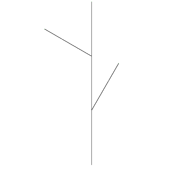
Iteration 0: (F)
Iteration 1: (F O(R30 F) F O(R-60 F) F)
Iteration 2: (F O(R30 F) F O(R-60 F) F O(R30 F O(R30 F) F O(R-60 F) F) F O(R30 F) F O(R-60 F) F O(R-60 F O(R30 F) F O(R-60 F) F) F O(R30 F) F O(R-60 F) F)
|
 Iteration 5 (with color) The Great Lambda Tree of Infinite Knowledge and Ultimate Power |


Note that L-system command rewriting is similar to the replacement rules in a BNF grammar. The important difference is that with L-system rewriting, each iteration replaces all instances of F in the initial string instead of just picking one to replace.
We can divide the problem of producing an L-system fractal into two main parts:
- Produce a list of L-system commands that represents the fractal by rewriting according to the L-system rule; and
- Drawing a list of L-system commands.
Representing L-System Commands
Here is a BNF grammar for L-system commands:
- CommandSequence ::= ( CommandList )
- CommandList ::= Command CommandList
- CommandList ::=
- Command ::= F
- Command ::= RAngle
- Command ::= OCommandSequence
- Angle ::= Number
We need to find a way to turn strings in this grammar into objects we can manipulate in a Scheme program. We can do this by looking at the BNF grammar, and converting the non-terminals into Scheme objects.
;;; CommandSequence ::= ( CommandList )
(define make-lsystem-command list)

;;; We represent the different commands as pairs where the first item in the
;;; pair is a tag that indicates the type of command: 'f for forward, 'r for
;;; rotate and 'o for offshoot.  We use quoted letters to make tags, which
;;; evaluate to the quoted letter.  The tag 'f is short for (quote f).

;;; Command ::= F
(define (make-forward-command) (cons 'f #f)) ;; No value, just use false.

;;; Command ::= RAngle
(define (make-rotate-command angle) (cons 'r angle))

;;; Command ::= OCommandSequence
(define (make-offshoot-command commandsequence) (cons 'o commandsequence))
- (is-forward? lcommand) — evaluates to #t if the parameter passed is a forward command (indicated by its first element being a 'f tag).
- (is-rotate? lcommand)
- (is-offshoot? lcommand)
- (get-angle lcommand) — evaluates to the angle associated with a rotate command. Produces an error if the command is not a rotate command (see below for how to produce an error).
- (get-offshoot-commands lcommand) — evaluates to the offshoot command list associated with an offshoot command. Produces an error if the command is not an offshoot command.
You will find the following procedures useful:
- (eq? v1 v2) — evaluates to #t if v1 and v2 are exactly the same; otherwise evaluates to false. For example, (eq? 's 's) evaluates to #t and (eq? 's 't) evaluates to #f.
- (error message) — produces an error with message a
string given as the first parameter. For example,
(error "Yikes! Attempt to get-angle for a command that is not an angle command")would display the message in red and stop execution. It is useful to use error in your code so you will more easily identify bugs. (Note: it is not necessary to use "Yikes!" in your error messages. For example, there is a strong contingent in favor of "Jinkies!")
You should be able to make up similar test cases yourself to make sure the other procedures you defined work.> (is-forward? (make-forward-command))
#t
> (is-forward? (make-rotate-command 90))
#f
> (get-angle (make-rotate-command 90))
90
> (get-angle (make-forward-command))
Yikes! Attempt to get-angle for a command that is not an angle command
New Special Forms
The code for this problem set uses three special forms that were not included in our original Scheme language description. None of the new special forms are necessary for expressing these programs — they could easily be rewritten using just the subset of Scheme introduced in Chapter 3 — but, as our programs get more complex it will be useful to use these expressions to make our programs shorter and clearer.
Begin Expression
The grammar rule for begin is:Expression ::= BeginExpressionThe evaluation rule for begin is:
BeginExpression ::= (begin MoreExpressions Expression)
Evaluation Rule 6: Begin. To evaluate (begin Expression1 Expression2 ... Expressionk), evaluate each sub-expression in order from left to right. The value of the begin expression is the value of Expressionk.The begin special form is useful when we are evaluating expressions that have side-effects. This means the expression is important not for the value it produces (since the begin expression ignores the values of all expressions except the last one), but for some change to the state of the machine it causes.
The special define syntax for procedures includes a hidden begin expression. The syntax,
   (define (Name Parameters)
       MoreExpressions Expression)
is an abbreviation for:
   (define name
       (lambda (Parameters)
          (begin MoreExpressions Expression)))
Let Expression
The grammar rule for let expressions is:Expression ::= LetExpressionThe evaluation rule for a let expression is:
LetExpression ::= (let (Bindings) Body)
Body ::= MoreExpressions Expression
Bindings ::= Binding Bindings
Bindings ::=
Binding ::= (Name Expression)
Evaluation Rule 7: Let. To evaluate a let expression, evaluate each binding in order. To evaluate each binding, evaluate the binding expression and bind the name to the value of that expression. Then, evaluate the body expressions in order with the names in the expression that match binding names substituted with their bound values. The value of the let expression is the value of the last body expression.A let expression can be transformed into an equivalent application expression. The let expression
(let ((Name1 Expression1)
      (Name2 Expression2)
      ...
      (Namek Expressionk))
    MoreExpressions Expression)
is equivalent to the application expression:
((lambda (Name1
          Name2
          ...
          Namek)
    (begin MoreExpressions Expression))
 Expression1
 Expression2
 ...
 Expressionk)
The advantage of the let expression syntax is it puts the expressions
next to the names to which they are bound. For example, the let
expression:
  (let ((a 2)
        (b (* 3 3)))
    (+ a b))
is easier to understand than the corresponding application expression:
((lambda (a b) (+ a b)) 2 (* 3 3))
Conditional Expression
Conditional expressions provide a way to concisely combine many decisions. The grammar rule for cond is:Expression ::= CondExpressionThe evaluation rule is:
CondExpression ::= (cond ClauseList)
ClauseList ::=
ClauseList ::= Clause ClauseList
Clause ::= (ExpressionTest ExpressionAction)
Clause ::= (else ExpressionAction)
Evaluation Rule 8: Conditionals. To evaluate a CondExpression, evaluate each clause's test expression in order until one is found that evaluates to a true value. Then, evaluate the action expression of that clause. The value of the CondExpression is the value of the action expression. If none of the test expressions evaluate to a true value, if the CondExpression includes an else clause, the value of the CondExpression is the value of the action expression associated with the else clause. If none of the test expressions evaluate to a true value, and the CondExpression has no else clause, the CondExpression has no value.Note that a conditional expression could straightforwardly be translated into an equivalent if expression:
   (cond (Test1 Action1)
         (Test2 Action2)
         ...
	 (Testk Actionk)
         (else Actionelse))
is equivalent to:
   (if Test1 Action1
       (if Test2 Action2
           ...
               (if Testk Actionk
                   actionelse)...))
Rewriting Curves
The power of the L-System commands comes from the rewriting mechanism. Recall how we described the tree fractal:Start: (F)To produce levels of the tree fractal, we need a procedure that takes a list of L-system commands and replaces each F command with the list of L-system commands given by the rule.
Rule: F ::= (F O(R30 F) F O(R-60 F) F)
So, for every command in the list:
- If the command is an F command, replace it with the replacement commands
- If the command is an RAngle command, keep it unchanged
- If the command is an OCommandSequence command, recursively rewrite every command in the offshoot's command list the same way
For example, consider a simple L-System rewriting:
Start: (F)We want to get:
Rule: F ::= (F R30 F)
Iteration1: (F R30 F)but if we just replace F's with (F R30 F) lists, we would get:
Iteration2: (F R30 F R30 F R30 F)
Iteration1: ((F R30 F))The easiest way to fix this problem is to flatten the result. The code should look similar to many recursive list procedures you have seen (this code is provided in lsystem.ss):
Iteration2: ((F R30 F) R30 (F R30 F))
(define (flatten-commands ll)
  (if (null? ll) ll
      (if (is-lsystem-command? (car ll))
	  (cons (car ll) (flatten-commands (cdr ll)))
	  (flat-append (car ll) (flatten-commands (cdr ll))))))

(define (flat-append lst ll)
  (if (null? lst) ll
      (cons (car lst) (flat-append (cdr lst) ll))))
Here's the easy part:
Complete the definition of rewrite-lcommands.(define (rewrite-lcommands lcommands replacement) (flatten-commands (map ; Procedure to apply to each command lcommands)))
We have pre-defined some simple lsystem commands (e.g., f, f-r30-f, f-f-r30) for easy testing. If you define these procedures correctly, you should produce these evaluations:
> (rewrite-lcommands f f-r30-f)
((f . #f) (r . 30) (f . #f))
> (rewrite-lcommands f-r30-f f-f-r30)
((f . #f) (f . #f) (r . 30) (r . 30) (f . #f) (f . #f) (r . 30))
To make interesting L-system curves, we will need to apply rewrite-lcommands many times. We will leave that until the last question. Next, we will work on turning sequences of L-system commands into curves we can draw.
Drawing L-System Fractals
To draw our L-system fractals, we will need procedures for drawing curves. There are many of different ways of thinking about curves. Mathematicians sometimes think about curves as functions from an x coordinate value to a y coordinate value. The problem with this way of thinking about curves is there can only be one y point for a given x point. This makes it impossible to make simple curves like a circle where there are two y points for every x value on the curve. So, a more useful way of thinking about curves is as functions from a number to a point. We can produce infinitely many different points on the curve by evaluating the curve function with the (infinitely many different) real numbers between 0 and 1 inclusive. Of course, we can't really evaluate the curve function at every value between 0 and 1. Instead, we will evaluate it at a large number of points distributed between 0 and 1 to display an approximation of the curve.
Points
We need a way to represent the points on our curves. A point is a pair of two values, x and y representing the horizontal and vertical location of the point.We will use a coordinate system from (0, 0) to (1, 1):
| (0.0, 1.0) | (1.0, 1.0) | ||
|
|
|||
| (0.0, 0.0) | (1.0, 0.0) |
Points have x and y coordinates. To represent points we would like to define procedures make-point, x-of-point and y-of-point. Our pictures will be more interesting if points can have color too. So, we represent a colored point using a list of three values: x, y and color:
(define (make-point x y) (list x y))
(define (make-colored-point x y c) (list x y c))
(define (is-colored-point? (= (length point) 3)

(define (x-of-point point) (car point))
(define (y-of-point point) (cadr point)) ;; (cadr x) = (car (cdr x))

;;; Regular points are black.  Colored points have a color.
(define (color-of-point point)
  (if (is-colored-point? point)
      (caddr point) ;; == (car (cdr (cdr point)))
      (make-color 0 0 0)))
Note that we have defined points so we can have both colored points and
colorless points that appear black.
We have provided some procedures for drawing on the window in graphics.ss:
- (window-draw-point point) — Draw the point on the window. For example, (window-draw-point (make-point 0.5 0.5)) will place a black dot in the center of the window. (The point is only one pixel, so it is hard to see.)
- (window-draw-line point0 point1) — Draw a black line from point0 to point1. For example, (window-draw-line (make-point 0.0 0.0) (make-point 1.0 1.0)) will draw a diagonal line from the bottom left corner to the top right corner.
Read through graphics.ss and look for other handy functions.
Drawing Curves
Building upon points, we can make curves and lines (straight lines are just a special kind of curve). Curves are procedures from values to points. One way to represent a curve is as a procedure that evaluates to a point for every value between 0.0 and 1.0. For example,
   (define (mid-line t)
      (make-point t 0.5))
defines a curve that is a horizontal line across the middle of the
window. If we apply mid-line to a value x, we get
the point (x, 0.5). Hence, if we apply
mid-line to all values between 0.0 and 1.0, we get a
horizontal line.
Predict what (x-of-point (mid-line 0.7)) and (y-of-point (mid-line 0.7)) should evaluate to. Try them in your Interactions window.
Of course, there are infinitely many values between 0.0 and 1.0, so we can't apply the curve function to all of them. Instead, we select enough values to show the curve well. To draw a curve, we need to apply the curve procedure to many values in the range from 0.0 to 1.0 and draw each point it evaluates to. Here's a procedure that does that:
  (define (draw-curve-points curve n)
    (define (draw-curve-worker curve t step)
      (if (<= t 1.0)
	   (begin
	     (window-draw-point (curve t))
	     (draw-curve-worker curve (+ t step) step))))
    (draw-curve-worker curve 0.0 (/ 1 n)))
The procedure draw-curve-points takes a procedure representing
a curve, and n, the number of points to draw. It
calls the draw-curve-worker procedure. The
draw-curve-worker procedure takes three parameters: a curve,
the current time step values, and the difference between time step
values. Hence, to start drawing the curve, draw-curve-points
evaluates draw-curve-worked with parameters curve
(to pass the same curve that was passed to
draw-curve-points), 0.0 (to start at the first
t value), and (/ 1 n) (to divide the time values
into n steps).
The draw-curve-worker procedure is defined recursively: if t is less than or equal to 1.0, we draw the current point using (window-draw-point (curve t)) and draw the rest of the points by evaluating (draw-curve-worker curve (+ t step) step)).
We stop once t is greater than 1.0, since we defined the curve over the interval [0.0, 1.0].
The draw-curve-worker code uses a being expression. The first expression in the begin expression is (window-draw-point (curve t)). The value it evaluates to is not important, what matters is the process of evaluating this expression draws a point on the display.
- Define a procedure, vertical-mid-line that can be passed to draw-curve-points so that (draw-curve-points vertical-mid-line 1000) produces a vertical line in the middle of the window.
- Define a procedure, make-vertical-line that takes one parameter and produces a procedure that produces a vertical line at that horizontal location. For example, (draw-curve-points (make-vertical-line 0.5) 1000) should produce a vertical line in the middle of the window and (draw-curve-points (make-vertical-line 0.2) 1000) should produce a vertical line near the left side of the window.
Manipulating Curves
The good thing about defining curves as procedures is it is easy to modify and combine then in interesting ways.For example, the procedure rotate-ccw takes a curve and rotates it 90 degrees counter-clockwise by swapping the x and y points:
(define (rotate-ccw curve)
  (lambda (t)
    (let ((ct (curve t)))
      (make-colored-point
       (- (y-of-point ct)) (x-of-point ct)
       (color-of-point ct)))))
We use a let expression here to avoid needing to evaluate (curve
t) more than once. It binds the value (curve t) evaluates
to, to the name ct.
Note that (rotate-ccw c) evaluates to a curve. The function rotate-ccw is a procedure that takes a procedure (a curve) and returns a procedure that is a curve.
Predict what (draw-curve-points (rotate-ccw mid-line) 1000) and (draw-curve-points (rotate-ccw (rotate-ccw mid-line)) 1000) will do. Confirm your predictions by trying them in your Interactions window.
Here's another example:
(define (shrink curve scale)
  (lambda (t)
    (let ((ct (curve t)))
      (make-colored-point
       (* scale (x-of-point ct))
       (* scale (y-of-point ct))
       (color-of-point ct)))))
Predict what (draw-curve-points (shrink mid-line .5)
1000) will do, and then try it in your Interactions window.
The shrink procedure doesn't produce quite what we want because in addition to changing the size of the curve, it moves it around. Why does this happen? Try shrinking a few different curves to make sure you understand why the curve moves.
One way to fix this problem is to center our curves around (0,0) and then translate them to the middle of the screen. We can do this by adding or subtracting constants to the points they produce:
(define (translate curve x y)
  (lambda (t)
    (let ((ct (curve t)))
      (make-colored-point
       (+ x (x-of-point ct)) (+ y (y-of-point ct))
       (color-of-point ct)))))
Now we have translate, it makes more sense to define
mid-line this way:
   (define (horiz-line t) (make-point t 0))
   (define mid-line (translate horiz-line 0 0.5))
When you are done, (draw-curve-points half-line 1000) should produce a horizontal line that starts in the middle of the window and extends to the right boundary.
Hint: If you do not see anything when you are drawing a curve, it may be that you haven't yet applied translate and the points are being drawn along the bottom edge of the screen.
In addition to altering the points a curve produces, we can alter a curve by changing the t values it will see. For example,
(define (first-half curve)
   (lambda (t) (curve (/ t 2))))
is a function that takes a curve and produces a new curve that is just the first half of the passed curve.
Predict what each of these expressions will do:
- (draw-curve-points (first-half mid-line) 1000)
- (draw-curve-points (first-half (first-half mid-line)) 1000)
The provided code includes several other functions that transform
curves including:
- (scale-x-y curve x-scale y-scale) — evaluates to curve stretched along the x and y axis by using the scale factors given
- (scale curve scale) — evaluates to curve stretched along the x and y axis by using the same scale factor
- (rotate-around-origin curve degrees) — evaluates to curve rotated counterclockwise by the given number of degrees.
It is also useful to have curve transforms where curves may be combined. An example is (connect-rigidly curve1 curve2) which evaluates to a curve that consists of curve1 followed by curve2. The starting point of the new curve is the starting point of curve1 and the end point of curve2 is the ending point of the new curve. Here's how connect-rigidly is defined:
(define (connect-rigidly curve1 curve2)
    (lambda (t)
      (if (< t (/ 1 2))
          (curve1 (* 2 t))
          (curve2 (- (* 2 t) 1)))))
Predict what (draw-curve-points (connect-rigidly vertical-mid-line
mid-line) 1000) will do. Is there any difference between that
and (draw-curve-points (connect-rigidly mid-line
vertical-mid-line) 1000)? Check your predictions in the
Interactions window.
Distributing t Values
The draw-curve-points procedure does not distribute the t-values evenly among connected curves, so the later curves appear dotty. This isn't too big a problem when only a few curves are combined; we can just increase the number of points passed to draw-curve-points to have enough points to make a smooth curve. In this problem set, however, you will be drawing curves made up of thousands of connected curves. Just increasing the number of points won't help much, as you'll see in Question 8.The way connect-rigidly is defined above, we use all the t-values below 0.5 on the first curve, and use the t-values between 0.5 and 1.0 on the second curve. If the second curve is the result of connecting two other curves, like (connect-rigidly c1 (connect-rigidly c2 c3)) then 50% of the points will be used to draw c1, 25% to draw c2 and 25% to draw c3.
(connect-rigidly c1 (connect-rigidly c2 (connect-rigidly curve3 (... cn))))The first argument to num-points is the number of t-values left. The second argument is the number of curves left.
Think about this yourself first, but look in ps3.ss for a hint if you are stuck. There are mathematical ways to calculate this efficiently, but the simplest way to calculate it is to define a procedure that keeps halving the number of points n times to find out how many are left for the nth curve.
Your num-points procedure should produce results similar to:
This means if we connected just 20 curves using connect-rigidly, and passed the result to draw-curve-points with one million as the number of points, there would still be only one or two points drawn for the 20th curve. If we are drawing thousands of curves, for most of them, not even a single point would be drawn!> (exact->inexact (num-points 1000 10))
1.953125
> (exact->inexact (num-points 1000 20))
0.0019073486328125
> (exact->inexact (num-points 1000000 20))
1.9073486328125
To fix this, we need to distribute the t-values between our curves more fairly. We have provided a procedure connect-curves-evenly in graphics.ss that connects a list of curves in a way that distributes the range of t values evenly between the curves.
The definition is a bit complicated, so don't worry if you don't understand it completely. You should, however, be able to figure out the basic idea for how it distributed the t-values evenly between every curve in a list of curves.
(define (connect-curves-evenly curvelist)
  (lambda (t)
    (let ((which-curve
	   (if (>= t 1.0) (- (length curvelist) 1)
	       (inexact->exact (floor (* t (length curvelist)))))))
      ((get-nth curvelist which-curve)
       (* (length curvelist)
	  (- t (* (/ 1 (length curvelist)) which-curve)))))))
It will also be useful to connect curves so that the next curve begins
where the first curve ends. We can do this by translating the second
curve to begin where the first curve ends. To do this for a list of
curves, we translate each curve in the list the same way using map:
(define (cons-to-curvelist curve curvelist)
  (let ((endpoint (curve 1.0))) ;; The last point in curve
    (cons curve
	  (map (lambda (thiscurve)
		 (translate thiscurve
                            (x-of-point endpoint) (y-of-point endpoint)))
	       curvelist))))
Drawing L-System Curves
To draw an L-system curve, we need to convert a sequence of L-system commands into a curve. We defined the connect-curves-evenly procedure to take a list of curves, and produce a single curve that connects all the curves. So, to draw an L-System curve, we need a procedure that turns an L-System Curve into a list of curve procedures.The convert-lcommands-to-curvelist procedure converts a list of L-System commands into a curve. Here is the code for convert-lcommands-to-curvelist (with some missing parts that you will need to complete). It will be explained later, but try to understand it yourself first.
(define (convert-lcommands-to-curvelist lcommands)
  (cond ((null? lcommands)
	 (list
	  ;;; We make a leaf with just a single point of green:
	  (lambda (t)
	    (make-colored-point 0.0 0.0 (make-color 0 255 0)))
	  ))
	((is-forward? (car lcommands))
	 (cons-to-curvelist
	  vertical-line
	  (convert-lcommands-to-curvelist (cdr lcommands))))
	((is-rotate? (car lcommands))
	      ;;; If this command is a rotate, every curve in the rest
	      ;;; of the list should should be rotated by the rotate angle
	 (let
	     ;; L-system turns are clockwise, so we need to use - angle
	     ((rotate-angle (- (get-angle (car lcommands)))))
	   (map
	    (lambda (curve)
              ;;; Question 9: fill this in
	      )
	     ;;; Question 9: fill this in
	    )))
	((is-offshoot? (car lcommands))
	 (append
  	  ;;; Question 10: fill this in
	  ))
	(#t (error "Bad lcommand!"))))
We define convert-lcommands-to-curvelist recursively. The base
case is when there are no more commands (the lcommands
parameter is null). It evaluates to the leaf curve (for now, we just
make a point of green — you may want to replace this with
something more interesting to make a better fractal). Since
convert-lcommands-to-curvelist evaluates to a list of
curves, we need to make a list of curves containing only one curve.
Otherwise, we need to do something different depending on what the first command in the command list is. If it is a forward command we draw a vertical line. The rest of the fractal is connected to the end of the vertical line using cons-to-curvelist. The recursive call to convert-lcommands-to-curve produces the curve list corresponding to the rest of the L-system commands. Note how we pass (cdr lcommands) in the recursive call to get the rest of the command list.
You can test your code by drawing the curve that results from any list of L-system commands that does not use offshoots. For example, evaluating
(draw-curve-points
   (position-curve
    (translate
     (connect-curves-evenly
      (convert-lcommands-to-curvelist
       (make-lsystem-command (make-rotate-command 150)
                             (make-forward-command)
                             (make-rotate-command -120)
                             (make-forward-command))))
     0.3 0.7)
    0 .5)
   10000)
should produce a "V".
Hint 1: See the next few paragraphs for help testing Question 10.
Hint 2: Evaluate tree-commands and look at its definition in lsystem.ss. This may help you to visualize relevant car and cdr combinations.
We have provided the position-curve procedure to make it easier to fit fractals into the graphics window:
(position-curve curve startx starty) — evaluates to a curve that translates curve to start at (startx, starty) and scales it to fit into the graphics window maintaining the aspect ratio (the x and y dimensions are both scaled the same amount)The code for position-curve is in curve.ss. You don't need to look at it, but should be able to understand it if you want to.
Now, you should be able to draw any l-system command list using position-curve and the convert-lcommands-to-curvelist function you completed in Questions 9 and 10. Try drawing a few simple L-system command lists before moving on to the next part. For example, given this input:
Your output should look like this:(draw-curve-points (position-curve (connect-curves-evenly (convert-lcommands-to-curvelist tree-commands)) 0.5 0.1) 50000)
Hint: You should use the rewrite-lcommands you defined in Question 5. You may also find it useful to use the n-times function (which we may have described in lecture):
(define (n-times proc n)
  (if (= n 1) proc
        (compose proc (n-times proc (- n 1)))))
(define (make-tree-fractal level)
  (make-lsystem-fractal tree-commands
			(make-lsystem-command (make-forward-command)) level))
(define (draw-lsystem-fractal lcommands)
  (draw-curve-points
   (position-curve
    (connect-curves-evenly (convert-lcommands-to-curvelist lcommands))
    0.5 0.1)
   50000))
For example, (draw-lsystem-fractal (make-tree-fractal 3)) will create a tree fractal with 3 levels of branching.
Draw some fractals by playing with the L-system commands. Try changing the rewrite rule, the starting commands, level and leaf curve (in convert-lcommands-to-curvelist) to draw an interesting fractal. You might want to make the branches colorful also. Try an make a fractal picture that will make a better course logo than the current Great Lambda Tree Of Infinite Knowledge and Ultimate Power.
To save your fractal in an image file, use the save-image procedure (defined in lsystem.ss). It can save images as .png files. For example, to save your fractal in yggdrasil.png evaluate
(save-image "yggdrasij.png")Especially ambitious students may find the Viewport Graphics documentation useful for enhancing your pictures.
(Everything below here is extra credit only.)
Extra Credit: Cognitive Psychology and Mental Rotation
 One of the great success stories in cognitive psychology is
the study of mental rotation — how humans rotate mental
representations of objects. If you consider the figures on the right,
with a bit of reasoning you should be able to confirm that you could
rotate the leftmost image in Figure 2 to form the second image in Figure 2
but not the third image in Figure 2. To get from the first image to the
third image, you'd need to flip or mirror it. As a more complicated
example, the leftmost three-dimensional image in Figure 1 cannot be rotated
in space to form the rightmost image — but this should take you
longer to verify. (If you're not quite certain what we mean by rotating a
three-dimensional image in space, click here
for an animation.)
One of the great success stories in cognitive psychology is
the study of mental rotation — how humans rotate mental
representations of objects. If you consider the figures on the right,
with a bit of reasoning you should be able to confirm that you could
rotate the leftmost image in Figure 2 to form the second image in Figure 2
but not the third image in Figure 2. To get from the first image to the
third image, you'd need to flip or mirror it. As a more complicated
example, the leftmost three-dimensional image in Figure 1 cannot be rotated
in space to form the rightmost image — but this should take you
longer to verify. (If you're not quite certain what we mean by rotating a
three-dimensional image in space, click here
for an animation.)
Cognitive psychologists, such as Roger Shepard and Jacqueline Metzler, have been interested in studying how humans manipulate mental representations of objects. To study this, they conducted a scientific experiment with a falsifiable hypothesis. In essence, their main hypothesis was that the time required to recognize that two perspective drawings portray objects of the same three-dimensional shape is found to be a linearly increasing function of the angular difference in the portrayed orientations of the two objects. To test this hypothesis, they presented subjects with a series of image pairs. Each pair of images was either one drawing and its rotation (as in Figure 2), or one drawing and another drawing that cannot be obtained from it by rotation (as in Figure 1). They then measured the time it took for human subjects to determine whether or not the two shapes were equivalent modulo rotation.
It turns out that the number of seconds it takes humans to determine if the images are rotations or not is a linear function of the angle of rotation. For example, if the angle is 40 degrees, it takes 2 seconds. If the angle is 60 degrees, it takes 3 seconds. If the angle is 80 degrees, it takes 4 seconds. In this example, it takes one second to reason about a 20 degree rotation.
There are many tasks in perception that take constant time. For example, detecting a red X against a random pattern of blue Os takes constant time, regardless of how many Os are present. Some aspects of perception are thus handled in parallel. The "linear function" result for mental rotation suggested that humans actually form a mental model of the object and rotate that model internally to see if it matches up with the other image. Subsequent experimentation with nuclear magnetic resonance and functional magnetic resonance imaging showed that there are particular areas of the brain associated with such mental rotation. Moreover, when a subject is performing a mental rotation tasks, mappings of which neurons are firing for shapes that themselves rotate over time.
This extra credit assignment involves reproducing parts of the original mental rotation experiment. The first part is to read Shepard and Metzler's Mental Rotation of Three-Dimensional Objects from Science volume 701, February 1971. It's only three pages long.
Eventually we will have datapoints from human subjects: rotational angles and the time taken to perform the task. We will want to analyze those datapoints to determine the slop of the line (as in Figure 2 of Shepard and Metzler's article). Write a function calculate-slope that takes a single argument: a list of datapoints. Each datapoint is a cons cell containing a rotation angle measurement and a time value measurement. Your function should return the average slope (rotation/time) for all of the datapoints.
For example:
In that dataset, it takes one second to reason about a 30.16 degree rotation.(define dataset (list (cons 32 1) (cons 54 2) (cons 95 3)))
(calculate-slope dataset)
30 1/6
We'll also need some way of getting timed user input. We'll assume a function get-timed-input that asks the user for a string and returns a pair containing the time taken and the string. You need not be able to write such a function, but you should be able to understand it:
The basic idea of the experiment is to present the user with a series of image pairs and record the times and answers. We'll use the following image:(define (get-timed-input) (let ((start-time (current-milliseconds)) (input (read-line (current-input-port))) (end-time (current-milliseconds))) (cons (- end-time start-time) input)))(get-timed-input)
y
(498 . "y")(get-timed-input)
n
(651 . "n")(get-timed-input)
y
(322 . "y")
Define a procedure run-mr-experiment that accepts a single parameter. That parameter is a list of cons cells. Each cons cell holds an angle in degrees and a boolean — the boolean is #t if the image should be flipped before being displayed. For each item in the list, you should clear the screen, display (mr-curve 0) on the left side of the screen, and display a rotated-and-possibly-flipped version of mr-curve on the right side of the screen based on the current list element. The user should enter "y" if it is a rotation and "n" if it is not (i.e., if a flip was involved). You should gather all of the times for which the user was correct as a dataset -- a list suitable for passing to (calculate-slope).(define (mr-curve degrees) (connect-curves-evenly (convert-lcommands-to-curvelist (make-lsystem-command (make-rotate-command degrees) (make-forward-command) (make-forward-command) (make-forward-command) (make-rotate-command 90) (make-forward-command) (make-rotate-command -90) (make-forward-command) (make-rotate-command -90) (make-forward-command) (make-forward-command) (make-rotate-command 90) (make-forward-command) (make-rotate-command 90) (make-forward-command) (make-forward-command) (make-forward-command) (make-rotate-command 90) (make-forward-command) (make-forward-command) (make-forward-command) (make-rotate-command 90) (make-forward-command) (make-rotate-command -90) (make-forward-command) (make-forward-command) (make-rotate-command 90) (make-forward-command) ))))
Hint: you may need to write your own version of position-curve to make this work.