CS150: Problem Set 3: L-System Fractals

Problem Set 3: L-System Fractals

Out: 5 February 2007
Due: Monday, 12 February 2007

Collaboration Policy - Read Carefully

For this problem set, you are required to work with an assigned partner. You will receive an email before midnight Monday containing the partner assignments. You and your partner should turn in one assignment with both of your names on it and both people must participate fully in all of the work and completely understand everything you submit. You should read the whole problem set yourself and think about the questions before beginning to work on them with your partner.

You may discuss this assignment with other students in the class and ask and provide help in useful ways. You may consult any outside resources you wish including books, papers, web sites and people except for materials from previous cs150 courses.

If you use resources other than the class materials, indicate what you used along with your answer.

Purpose

Practice programming with recursive definitions and procedures
Explore the power of rewrite rules
Write recursive functions that manipulate lists
Make a cs150 course logo better than "The Great Lambda Tree of Infinite Knowledge and Ultimate Power"

Download: Download ps3.zip to your machine and unzip it into your home directory J:\cs150\ps3. This file contains:

ps3.scm — A template for your answers. You should do the problem set by editing this file.
graphics.scm — Scheme code for drawing curves.
lsystem.scm — provided incomplete code for producing L-System Fractals

Unlike in Problem Set 1 and Problem Set 2, you are expected to be able to understand all the code provided for this problem set (and all future problem sets in this class unless specifically explained otherwise). This problem set expects you to write considerably more code than Problem Set 2. We recommend you start early and take advantage of the staffed lab hours.

Background

In this problem set, you will explore a method of creating fractals known as the Lindenmayer system (or L-system). Aristid Lindemayer, a theoretical biologist at the University of Utrecht, developed the L-system in 1968 as a mathematical theory of plant development. In the late 1980s, he collaborated with Przemyslaw Prusinkiewicz, a computer scientist at the University of Regina, to explore computational properties of the L-system and developed many of the ideas on which this problem set is based.

The idea behind L-system fractals is that we can describe a curve as a list of lines and turns, and create new curves by rewriting old curves. Everything in an L-system curve is either a forward line (denoted by F), or a right turn (denoted by Ra where a is an angle in degrees clockwise). We can denote left turns by using negative angles.

We create fractals by recursively replacing all forward lines in a curve list with the original curve list. Lindemayer found that many objects in nature could be described using regularly repeating patterns. For example, the way some tree branches sprout from a trunck can be described using the pattern: F O(R30 F) F O(R-60 F) F. This is interpreted as: the trunk goes up one unit distance, a branch sprouts at an angle 30 degrees to the trunk and grows for one unit. The O means an offshoot — we draw the curve in the following parentheses, and then return to where we started before the offshoot. The trunk grows another unit and now another branch, this time at -60 degrees relative to the trunk grows for one units. Finally the trunk grows for one more unit. The branches continue to sprout in this manner as they get smaller and smaller, and eventually we reach the leaves.

We can describe this process using replacement rules:

Start: (F)
Rule: F ::= (F O(R30 F) F O(R-60 F) F)

Here are the commands this produces after two iterations:

Iteration 0: (F)
Iteration 1: (F O(R30 F) F O(R-60 F) F)
Iteration 2: (F O(R30 F) F O(R-60 F) F O(R30 F O(R30 F) F O(R-60 F) F) F O(R30 F) F O(R-60 F) F O(R-60 F O(R30 F) F O(R-60 F) F) F O(R30 F) F O(R-60 F) F)

Here's what that looks like:

Iteration 0

Iteration 1

Iteration 2

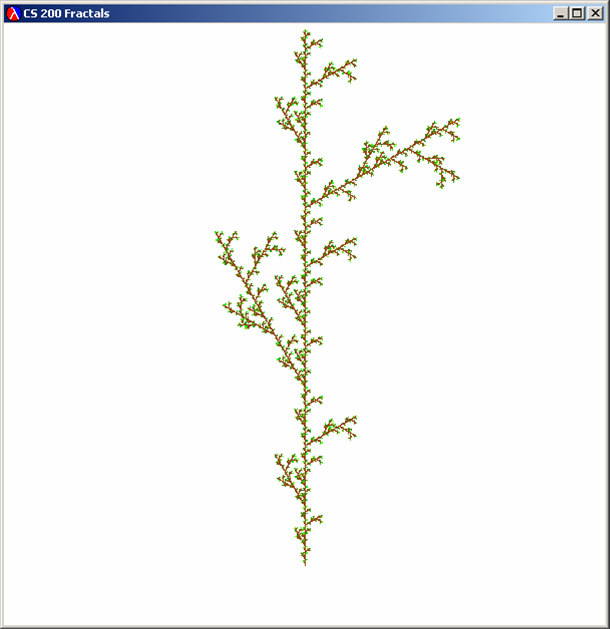Iteration 5

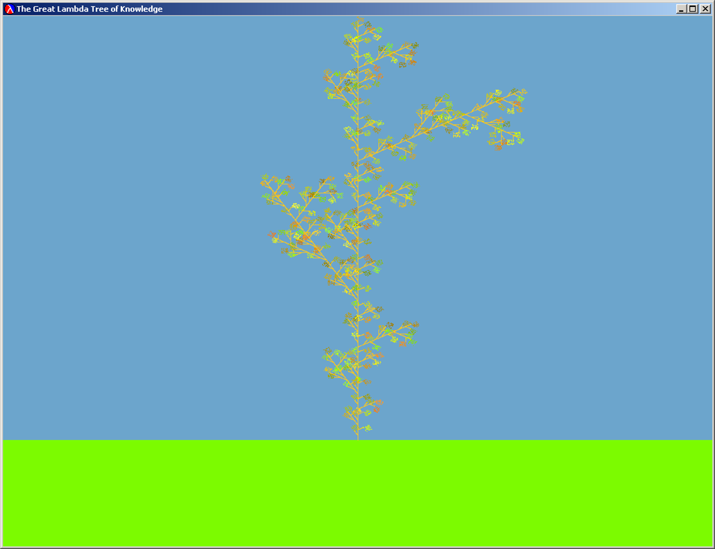Iteration 5 (with color)
The Great Lambda Tree of
Infinite Knowledge and Ultimate Power

Note that L-system command rewriting is similar to the replacement rules in a BNF grammar. The important difference is that with L-system rewriting, each iteration replaces all instances of F in the initial string instead of just picking one to replace.

We can divide the problem of producing an L-system fractal into two main parts:

Produce a list of L-system commands that represents the fractal by rewriting according to the L-system rule; and
Drawing a list of L-system commands.

We will first work on producing the list of L-system commands, and then work on how to draw a list of L-system commands.

Representing L-System Commands

Here is a BNF grammar for L-system commands:

CommandSequence ::= ( CommandList )

CommandList ::= Command CommandList

CommandList ::=

Command ::= F

Command ::= RAngle

Command ::= OCommandSequence

Angle ::= Number

Question 1: Show that (F O(R-60 F) F) is a string in the language defined by our BNF grammar. To do this, you should start with CommandSequence, and show a sequence of replacements that follow the grammar rules that produce the target string. You can use the rule numbers above to identify the rules.

We need to find a way to turn strings in this grammar into objects we can manipulate in a Scheme program. We can do this by looking at the BNF grammar, and converting the non-terminals into Scheme objects.

;;; CommandSequence ::= ( CommandList )
(define make-lsystem-command list)

;;; We represent the different commands as pairs where the first item in the
;;; pair is a tag that indicates the type of command: 'f for forward, 'r for
;;; rotate and 'o for offshoot.  We use quoted letters to make tags, which 
;;; evaluate to the quoted letter.  The tag 'f is short for (quote f).

;;; Command ::= F
(define (make-forward-command) (cons 'f #f)) ;; No value, just use false.

;;; Command ::= RAngle
(define (make-rotate-command angle) (cons 'r angle))

;;; Command ::= OCommandSequence
(define (make-offshoot-command commandsequence) (cons 'o commandsequence))

Question 2: It will be useful to have procedures that take L-system commands as parameters, and return information about those commands. Define the following procedures in ps3.scm:

(is-forward? lcommand) — evaluates to #t if the parameter passed is a forward command (indicated by its first element being a 'f tag).
(is-rotate? lcommand)
(is-offshoot? lcommand)
(get-angle lcommand) — evaluates to the angle associated with a rotate command. Produces an error if the command is not a rotate command (see below for how to produce an error).
(get-offshoot-commands lcommand) — evaluates to the offshoot command list associated with an offshoot command. Produces an error if the command is not an offshoot command.

You will find the following procedures useful:

(eq? v1 v2) — evaluates to #t if v1 and v2 are exactly the same; otherwise evaluates to false. For example, (eq? 's 's) evaluates to #t and (eq? 's 't) evaluates to #f.
(error message) — produces an error with message a string given as the first parameter. For example,
(error "Yikes! Attempt to get-angle for a command that is not an angle command")
would display the message in red and stop execution. It is useful to use error in your code so you will more easily identify bugs. (Note: it is not necessary to use "Yikes!" in your error messages.)

If you define these procedures correctly, you should produce these evaluations:

> (is-forward? (make-forward-command))

#t

> (is-forward? (make-rotate-command 90))

#f

> (get-angle (make-rotate-command 90))

90

> (get-angle (make-forward-command))

Yikes! Attempt to get-angle for a command that is not an angle command

You should be able to make up similar test cases yourself to make sure the other procedures you defined work.

New Special Forms

The code for this problem set uses three special forms that were not included in our original Scheme language description. None of the new special forms are necessary for expressing these programs — they could easily be rewritting using just the subset of Scheme introduced in Chapter 3 — but, as our programs get more complex it will be useful to use these expressions to make our programs shorter and clearer.

Begin Expression

The grammar rule for begin is:

Expression ::= BeginExpression
BeginExpression ::= (begin MoreExpressions Expression)

The evaluation rule for begin is:

Evaluation Rule 6: Begin. To evaluate (begin Expression₁ Expression₂ ... Expression_k), evaluate each sub-expression in order from left to right. The value of the begin expression is the value of Expression_k.

The begin special form is useful when we are evaluating expressions that have side-effects. This means the expression is important not for the value it produces (since the begin expression ignores the values of all expressions except the last one), but for some change to the state of the machine it causes.

The special define syntax for procedures includes a hidden begin expression. The syntax,

   (define (Name Parameters) 
       MoreExpressions Expression)

is an abbreviation for:

   (define name
       (lambda (Parameters) 
          (begin MoreExpressions Expression)))

Let Expression

The grammar rule for let expressions is:

Expression ::= LetExpression
LetExpression ::= (let (Bindings) Body)
Body ::= MoreExpressions Expression
Bindings ::= Binding Bindings
Bindings ::=
Binding ::= (Name Expression)

The evaluation rule for a let expression is:

Evaluation Rule 7: Let. To evaluate a let expression, evaluate each binding in order. To evaluate each binding, evaluate the binding expression and bind the name to the value of that expression. Then, evaluate the body expressions in order with the names in the expression that match binding names subsituted with their bound values. The value of the let expression is the value of the last body expression.

A let expression can be transformed into an equivalent application expression. The let expression

(let ((Name₁ Expression₁) 
      (Name₂ Expression₂) 
      ...
      (Name_k Expression_k))
    MoreExpressions Expression)

is equivalent to the application expression:

((lambda (Name₁ 
          Name₂
          ... 
          Name_k)
    (begin MoreExpressions Expression))
 Expression₁ 
 Expression₂
 ... 
 Expression_k)

The advantage of the let expression syntax is it puts the expressions next to the names to which they are bound. For example, the let expression:

  (let ((a 2)
        (b (* 3 3)))
    (+ a b))

is easier to understand than the corresponding application expression:

   ((lambda (a b) (+ a b)) 2 (* 3 3))

Conditional Expression

Conditional expressions provide a way to condensly combine many decisions. The grammar rule for cond is:

Expression ::= CondExpression
CondExpression ::= (cond ClauseList)
ClauseList ::=
ClauseList ::= Clause ClauseList
Clause ::= (Expression_Test Expression_Action)
Clause ::= (else Expression_Action)

The evaluation rule is:

Evaluation Rule 8: Conditionals. To evaluate a CondExpression, evaluate each clause's test expression in order until one is found that evaluates to a true value. Then, evaluate the action expression of that clause. The value of the CondExpression is the value of the action expression. If none of the test expressions evaluate to a true value, if the CondExpression includes an else clause, the value of the CondExpression is the value of the action expression associated with the else clause. If none of the test expressions evaluate to a true value, and the CondExpression has no else clause, the CondExpression has no value.

Note that a conditional expression could straightforwardly be translated into an equivalent if expression:

   (cond (Test₁ Action₁)
         (Test₂ Action₂)
         ...
	 (Test_k Action_k)
         (else Action_else))

is equivalent to:

   (if Test₁ Action₁
       (if Test₂ Action₂
           ...
               (if Test_k Action_k
                   action_else)...))

Question 3: Demonstrate how any if expression can be rewritten as an equivalent conditional expression. A convincing demonstration would include a transformation similar to the one we showed for transforming a conditional expression into an equivalent if expression, but that transforms an if expression into the equivalent cond expression.

Question 4: Is the begin expression necessary? Either explain how to obtain the same exact behavior as (begin Expr₁ Expr₂) without using begin, or explain why it is not possible to obtain the same behavior using only the subset of Scheme defined in Chapter 3.

Rewriting Curves

The power of the L-System commands comes from the rewriting mechanism. Recall how we described the tree fractal:

Start: (F)
Rule: F ::= (F O(R30 F) F O(R-60 F) F)

To produce levels of the tree fractal, we need a procedure that takes a list of L-system commands and replaces each F command with the list of L-system commands given by the rule.

So, for every command in the list:

If the command is an F command, replace it with the replacement commands
If the command is an RAngle command, keep it unchanged
If the command is an OCommandSequence command, recursively rewrite every command in the offshoot's command list the same way

One slight complication is that the replacement commands are a list of L-system commands, and we want to end up with a flat list of L-System commands.

For example, consider a simple L-System rewriting:

Start: (F)
Rule: F ::= (F R30 F)

We want to get:

Iteration1: (F R30 F)
Iteration2: (F R30 F R30 F R30 F)

but if we just replace F's with (F R30 F) lists, we would get:

Iteration1: ((F R30 F))
Iteration2: ((F R30 F) R30 (F R30 F))

The easiest way to fix this problem is to flatten the result. The code should look similar to many recursive list procedures you have seen (this code is provided in lsystem.scm):

(define (flatten-commands ll)
  (if (null? ll) ll
      (if (is-lsystem-command? (car ll))
	  (cons (car ll) (flatten-commands (cdr ll)))
	  (flat-append (car ll) (flatten-commands (cdr ll))))))

(define (flat-append lst ll)
  (if (null? lst) ll
      (cons (car lst) (flat-append (cdr lst) ll))))

Question 5: Define a procedure rewrite-lcommands in ps3.scm that takes a list of L-system commands as its first parameter. The second parameter is a list of L-system commands that should replace every forward command in the first list of commands in the result.

Here's the easy part:

(define (rewrite-lcommands lcommands replacement)
  (flatten-commands
   (map 
   ; Procedure to apply to each command
   lcommands)))

Complete the definition of rewrite-lcommands.

To make interesting L-system curves, we will need to apply rewrite-lcommands many times. We will leave that until the last question. Next, we will work on turning sequences of L-system commands into curves we can draw.

Drawing L-System Fractals

To draw our L-system fractals, we will need procedures for drawing curves. There are many of different ways of thinking about curves. Mathematicians sometimes think about curves as functions from an x coordinate value to a y coordinate value. The problem with this way of thinking about curves is there can only be one y point for a given x point. This makes it impossible to make simple curves like a circle where there are two y points for every x value on the curve. So, a more useful way of thinking about curves is as functions from a number to a point. We can produce infinitely many different points on the curve by evaluating the curve function with the (infinitely many different) real numbers between 0 and 1 inclusive. Of course, we can't really evaluate the curve function at every value between 0 and 1. Instead, we will evaluate it at a large number of points distributed between 0 and 1 to display an approximation of the curve.

Points

We need a way to represent the points on our curves. A point is a pair of two values, x and y representing the horizontal and vertical location of the point.

We will use a coordinate system from (0, 0) to (1, 1):

(0.0, 1.0)

(1.0, 1.0)

(0.0, 0.0)

(1.0, 0.0)

Points have x and y coordinates. To represent points we would like to define procedures make-point, x-of-point and y-of-point. Our pictures will be more interesting if points can have color too. So, we represent a colored point using a list of three values: x, y and color:

(define (make-point x y) (list x y))
(define (make-colored-point x y c) (list x y c))
(define (is-colored-point? (= (length point) 3)

(define (x-of-point point) (car point))
(define (y-of-point point) (cadr point)) ;; (cadr x) = (car (cdr x))

;;; Regular points are black.  Colored points have a color.
(define (color-of-point point)
  (if (is-colored-point? point)
      (caddr point) ;; == (car (cdr (cdr point)))
      (make-color 0 0 0)))

Note that we have defined points so we can have both colored points and colorless points that appear black.

We have provided some procedures for drawing on the window in graphics.scm:

(window-draw-point point) — Draw the point on the window. For example, (window-draw-point (make-point 0.5 0.5)) will place a black dot in the center of the window. (The point is only one pixel, so it is hard to see.)
(window-draw-line point0 point1) — Draw a black line from point0 to point1. For example, (window-draw-line (make-point 0.0 0.0) (make-point 1.0 1.0)) will draw a diagonal line from the bottom left corner to the top right corner.

Drawing Curves

Building upon points, we can make curves and lines (straight lines are just a special kind of curve). Curves are procedures from values to points. One way to represent a curve is as a procedure that evaluates to a point for every value between 0.0 and 1.0. For example,

   (define (mid-line t)
      (make-point t 0.5))

defines a curve that is a horizontal line across the middle of the window. If we apply mid-line to a value x, we get the point (x, 0.5). Hence, if we apply mid-line to all values between 0.0 and 1.0, we get a horizontal line.

Predict what (x-of-point (mid-line 0.7)) and (y-of-point (mid-line 0.7)) should evaluate to. Try them in your Interactions window.

Of course, there are infinitely many values between 0.0 and 1.0, so we can't apply the curve function to all of them. Instead, we select enough values to show the curve well. To draw a curve, we need to apply the curve procedure to many values in the range from 0.0 to 1.0 and draw each point it evaluates to. Here's a procedure that does that:

  (define (draw-curve-points curve n)
    (define (draw-curve-worker curve t step)
      (if (<= t 1.0)
	   (begin
	     (window-draw-point (curve t))
	     (draw-curve-worker curve (+ t step) step))))
    (draw-curve-worker curve 0.0 (/ 1 n)))

The procedure draw-curve-points takes a procedure representing a curve, and n, the number of points to draw. It calls the draw-curve-worker procedure. The draw-curve-worker procedure takes three parameters: a curve, the current time step values, and the difference between time step values. Hence, to start drawing the curve, draw-curve-points evaluates draw-curve-worked with parameters curve (to pass the same curve that was passed to draw-curve-points), 0.0 (to start at the first t value), and (/ 1 n) (to divide the time values into n steps).

The draw-curve-worker procedure is defined recursively: if t is less than or equal to 1.0, we draw the current point using (window-draw-point (curve t)) and draw the rest of the points by evaluating (draw-curve-worker curve (+ t step) step)).

We stop once t is greater than 1.0, since we defined the curve over the interval [0.0, 1.0].

The draw-curve-worker code uses a being expression. The first expression in the begin expression is (window-draw-point (curve t)). The value it evaluates to is not important, what matters is the process of evaluating this expression draws a point on the display.

Question 6:

Define a procedure, vertical-mid-line that can be passed to draw-curve-points so that (draw-curve-points vertical-mid-line 1000) produces a vertical line in the middle of the window.
Define a procedure, make-vertical-line that takes one parameter and produces a procedure that produces a vertical line at that horizontal location. For example, (draw-curve-points (make-vertical-line 0.5) 1000) should produce a vertical line in the middle of the window and (draw-curve-points (make-vertical-line 0.2) 1000) should produce a vertical line near the left side of the window.

Manipulating Curves

The good thing about defining curves as procedures is it is easy to modify and combine then in interesting ways.

For example, the procedure rotate-ccw takes a curve and rotates it 90 degrees counter-clockwise by swapping the x and y points:

(define (rotate-ccw curve)
  (lambda (t)
    (let ((ct (curve t)))
      (make-colored-point
       (- (y-of-point ct)) (x-of-point ct)
       (color-of-point ct)))))

We use a let expression here to avoid needing to evaluate (curve t) more than once. It binds the value (curve t) evaluates to, to the name ct.

Note that (rotate-ccw c) evaluates to a curve. The function rotate-ccw is a procedure that takes a procedure (a curve) and returns a procedure that is a curve.

Predict what (draw-curve-points (rotate-ccw mid-line) 1000) and (draw-curve-points (rotate-ccw (rotate-ccw mid-line)) 1000) will do. Confirm your predictions by trying them in your Interactions window.

Here's another example:

(define (shrink curve scale)
  (lambda (t)
    (let ((ct (curve t)))
      (make-colored-point
       (* scale (x-of-point ct))
       (* scale (y-of-point ct))
       (color-of-point ct)))))

Predict what (draw-curve-points (shrink mid-line .5) 1000) will do, and then try it in your Interactions window.

The shrink procedure doesn't produce quite what we want because in addition to changing the size of the curve, it moves it around. Why does this happen? Try shrinking a few different curves to make sure you understand why the curve moves.

One way to fix this problem is to center our curves around (0,0) and then translate them to the middle of the screen. We can do this by adding or subtracting constants to the points they produce:

(define (translate curve x y)
  (lambda (t)
    (let ((ct (curve t)))
      (make-colored-point
       (+ x (x-of-point ct)) (+ y (y-of-point ct))
       (color-of-point ct)))))

Now we have translate, it makes more sense to define mid-line this way:

   (define (horiz-line t) (make-point t 0))
   (define mid-line (translate horiz-line 0 0.5))

Question 7: To check you understand everything so far, define a procedures draw-half-line that uses translate, horiz-line and shrink to draw a line half the width of the window that is centered in the middle of the display window.

In addition to altering the points a curve produces, we can alter a curve by changing the t values it will see. For example,

(define (first-half curve)
   (lambda (t) (curve (/ t 2))))

is a function that takes a curve and produces a new curve that is just the first half of the passed curve.

Predict what each of these expressions will do:

(draw-curve-points (first-half mid-line) 1000)
(draw-curve-points (first-half (first-half mid-line)) 1000)

Try evaluating them in your Interactions window to check if you were right. (Remember to use (clear-window) to clear the display window so you can see the new curve without the old one.)

The provided code includes several other functions that transform curves including:

(scale-x-y curve x-scale y-scale) — evalutes to curve stretched along the x and y axis by using the scale factors given
(scale curve scale) — evaluates to curve stretched along the x and y axis by using the same scale factor
(rotate-around-origin curve degrees) — evaluates to curve rotated counterclockwise by the given number of degrees.

You should be able to understand the code in graphics.scm that defines these functions.

It is also useful to have curve transforms where curves may be combined. An example is (connect-rigidly curve1 curve2) which evaluates to a curve that consists of curve1 followed by curve2. The starting point of the new curve is the starting point of curve1 and the end point of curve2 is the ending point of the new curve. Here's how connect-rigidly is defined:

(define (connect-rigidly curve1 curve2)
    (lambda (t)
      (if (< t (/ 1 2))
          (curve1 (* 2 t))
          (curve2 (- (* 2 t) 1)))))

Predict what (draw-curve-points (connect-rigidly vertical-mid-line mid-line) 1000) will do. Is there any difference between that and (draw-curve-points (connect-rigidly mid-line vertical-mid-line) 1000)? Check your predictions in the Interactions window.

Distributing `t` Values

The draw-curve-points procedure does not distribute the t-values evenly among connected curves, so the later curves appear dotty. This isn't too big a problem when only a few curves are combined; we can just increase the number of points passed to draw-curve-points to have enough points to make a smooth curve. In this problem set, however, you will be drawing curves made up of thousands of connected curves. Just increasing the number of points won't help much, as you'll see in Question 8.

The way connect-rigidly is defined above, we use all the t-values below 0.5 on the first curve, and use the t-values between 0.5 and 1.0 on the second curve. If the second curve is the result of connecting two other curves, like (connect-rigidly c1 (connect-rigidly c2 c3)) then 50% of the points will be used to draw c1, 25% to draw c2 and 25% to draw c3.

Question 8: Define a procedure num-points that determines the approximate number of t-values that will be used for the n^th curve when drawing

   (connect-rigidly c1 (connect-rigidly c2 (connect-rigidly curve3 (... cn))))

Think about this yourself first, but look in ps3.scm for a hint if you are stuck. There are mathematical ways to calculate this efficiently, but the simplest way to calculate it is to define a procedure that keeps halving the number of points n times to find out how many are left for the n^th curve.

Your num-points procedure should produce results similar to:

> (exact->inexact (num-points 1000 10))

1.95

> (exact->inexact (num-points 1000 20))

0.0019073486328125

> (exact->inexact (num-points 1000000 20))

1.9073486328125

This means if we connected just 20 curves using connect-rigidly, and passed the result to draw-curve-points with one million as the number of points, there would still be only one or two points drawn for the 20^th curve. If we are drawing thousands of curves, for most of them, not even a single point would be drawn!

To fix this, we need to distribute the t-values between our curves more fairly. We have provided a procedure connect-curves-evenly in graphics.scm that connects a list of curves in a way that distributes the range of t values evenly between the curves.

The definition is a bit complicated, so don't worry if you don't understand it completely. You should, however, be able to figure out the basic idea for how it distributed the t-values evenly between every curve in a list of curves.

(define (connect-curves-evenly curvelist)
  (lambda (t)
    (let ((which-curve
	   (if (>= t 1.0) (- (length curvelist) 1)
	       (inexact->exact (floor (* t (length curvelist)))))))
      ((get-nth curvelist which-curve)
       (* (length curvelist)
	  (- t (* (/ 1 (length curvelist)) which-curve)))))))

It will also be useful to connect curves so that the next curve begins where the first curve ends. We can do this by translating the second curve to begin where the first curve ends. To do this for a list of curves, we translate each curve in the list the same way using map:

(define (cons-to-curvelist curve curvelist)
  (let ((endpoint (curve 1.0))) ;; The last point in curve
    (cons curve
	  (map (lambda (thiscurve)
		 (translate thiscurve 
                            (x-of-point endpoint) (y-of-point endpoint)))
	       curvelist))))

Drawing L-System Curves

To draw an L-system curve, we need to convert a sequence of L-system commands into a curve. We defined the connect-curves-evenly procedure to take a list of curves, and produce a single curve that connects all the curves. So, to draw an L-System curve, we need a procedure that turns an L-System Curve into a list of curve procedures.

The convert-lcommands-to-curvelist procedure converts a list of L-System commands into a curve. Here is the code for convert-lcommands-to-curvelist (with some missing parts that you will need to complete). It will be explained later, but try to understand it yourself first.

(define (convert-lcommands-to-curvelist lcommands)
  (cond ((null? lcommands)
	 (list 
	  ;;; We make a leaf with just a single point of green:
	  (lambda (t) 
	    (make-colored-point 0.0 0.0 (make-color 0 255 0))) 
	  ))
	((is-forward? (car lcommands))
	 (cons-to-curvelist
	  vertical-line
	  (convert-lcommands-to-curvelist (cdr lcommands))))
	((is-rotate? (car lcommands))
	      ;;; If this command is a rotate, every curve in the rest 
	      ;;; of the list should should be rotated by the rotate angle
	 (let
	     ;; L-system turns are clockwise, so we need to use - angle
	     ((rotate-angle (- (get-angle (car lcommands)))))
	   (map
	    (lambda (curve)
              ;;; Question 9: fill this in
	      )
	     ;;; Question 9: fill this in
	    )))
	((is-offshoot? (car lcommands))
	 (append
  	  ;;; Question 10: fill this in
	  ))
	(#t (error "Bad lcommand!"))))

We define convert-lcommands-to-curvelist recursively. The base case is when there are no more commands (the lcommands parameter is null). It evaluates to the leaf curve (for now, we just make a point of green — you may want to replace this with something more interesting to make a better fractal). Since convert-lcommands-to-curvelist evaluates to a list of curves, we need to make a list of curves containing only one curve.

Otherwise, we need to do something different depending on what the first command in the command list is. If it is a forward command we draw a vertical line. The rest of the fractal is connected to the end of the vertical line using cons-to-curvelist. The recursive call to convert-lcommands-to-curve produces the curve list corresponding to the rest of the L-system commands. Note how we pass (cdr lcommands) in the recursive call to get the rest of the command list.

Question 9: Fill in the missing code for handling rotate commands (marked as Question 9 in ps3.scm). You will want to use (rotate-around-origin curve rotate-angle) somewhere in your code to rotate every curve after the rotate command by the rotate-angle.

You can test your code by drawing the curve that results from any list of L-system commands that does not use offshoots. For example, evaluating

(draw-curve-points
   (position-curve
    (translate
     (connect-curves-evenly
      (convert-lcommands-to-curvelist
       (make-lsystem-command (make-rotate-command 150)
                             (make-forward-command)
                             (make-rotate-command -120)
                             (make-forward-command))))
     0.3 0.7)
    0 .5)
   10000)

should produce a "V".

Question 10: Fill in the missing code for handling offshoot commands (marked as Question 10 in ps3.scm).

We have provided the position-curve procedure to make it easier to fit fractals onto the graphics window:

(position-curve curve startx starty) — evaluates to a curve that translates curve to start at (startx, starty) and scales it to fit into the graphics window maintaining the aspect ratio (the x and y dimensions are both scaled the same amount)

The code for position-curve is in curve.scm. You don't need to look at it, but should be able to understand it if you want to.

Now, you should be able to draw any l-system command list using position-curve and the convert-lcommands-to-curvelist function you completed in Questions 9 and 10. Try drawing a few simple L-system command lists before moving on to the next part.

Question 11: Define a procedure make-lsystem-fractal in ps3.scm that takes three parameters: replace-commands, a list of L-system commands that replace forward commands in the rewriting; start, a list of L-system commands that describes the starting curve; level, the number of iterations to apply the rewrite rule.

Hint: You should use the rewrite-lcommands you defined in Question 5. You may also find it useful to use the n-times function from lecture.

You should be able to draw a tree fractal using make-tree-fractal and draw-lsystem-fractal (these and the tree-commands list of L-system commands are defined in lsystem.scm):

(define (make-tree-fractal level)
  (make-lsystem-fractal tree-commands 
			(make-lsystem-command (make-forward-command)) level))

(define (draw-lsystem-fractal lcommands)
  (draw-curve-points 
   (position-curve 
    (connect-curves-evenly (convert-lcommands-to-curvelist lcommands)) 
    0.5 0.1) 
   50000))

For example, (draw-lsystem-fractal (make-tree-fractal 3)) will create a tree fractal with 3 levels of branching.

Draw some fractals by playing with the L-system commands. Try changing the rewrite rule, the starting commands, level and leaf curve (in convert-lcommands-to-curvelist) to draw an interesting fractal. You might want to make the branches colorful also. Try an make a fractal picture that will make a better course logo than the current Great Lambda Tree Of Infinite Knowledge and Ultimate Power.

To save your fractal in an image file, use the save-image procedure (defined in lsystem.scm). It can save images as .png files. For example, to save your fractal in wondertree.png evaluate

(save-image "wondertree.png")

Especially ambitious students may find the Viewport Graphics documentation useful for enhancing your pictures.

Question 12: Submit your best fractal images and the code you used to create them using the fractal submission page. The best pictures will appear on the course web page and will be rewarded with untold fame, invaluable fortune and maybe even a double gold star on this problem set.

Credits: This problem set was originally created for CS200 Spring 2002 by Dante Guanlao, Jon Erdman and David Evans, and revised for CS200 Spring 2003 by Jacques Fournier and David Evans, and revised for CS200 Spring 2004, CS150 Fall 2005, and CS150 Spring 2007 by David Evans. A version of this assignment was also used at the University of Georgia.