| Problem Set 2: Function Fractals |
Out: 25 January 2002 Due: 4 February 2002, before class |
Turn-in Checklist:
On February 4, bring to class a stapled turn in containing:
|
Collaboration Policy - Read Carefully
For this problem set, you may either work alone and turn in a problem set with just your name on it, or work with one other student in the class of your choice. If you work with a partner, you and your partner should turn in one assignment with both of your names on it.PurposeRegardless of whether you work alone or with a partner, you are encouraged to discuss this assignment with other students in the class and ask and provide help in useful ways. You may consult any outside resources you wish including books, papers, web sites and people. If you use resources other than the class materials, indicate what you used along with your answer.
- Become comfortable with procedures as parameters and results.
- Get some practice defining recursive procedures.
- Play (nicely) with fractals.
| Unlike in Problem Set 1, you are expected to be able to understand all the code provided for this problem set (and all future problem sets in this class unless specifically explained otherwise). This problem set requires less reading and introduces fewer new ideas than Problem Set 1, but expects you to write more code. As always, we recommend you start early and take advantage of staffed lab hours. |
Background
The name "fractal" was invented by Benoit Mandlebrot from the Latin adtive fractus, meaning to break (as in fracture). A fractal is a geometric shape that can be recursively broken down into smaller parts. Unlike a mosaic, the smaller parts of a fractal all look like the original shape, just scaled down. There are many fractal-like structures found in the real world including clouds, coastlines, trees and stock market fluctuations.
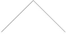
Fractals receive a lot of attention because of their interesting mathematical properties, but mainly because they look really cool. There are several types of fractals but the fractal we’ll be working with in this assignment is the Gosper Curve (you'll see a few more in PS3), pictures created by the repetition of a simple process. At every iteration of the Gosper curve, an approximation to the fractal curve is made, the next iteration consists of two scaled-down copies of the current iteration, rotated 45 degrees, and connected end to end.
 |
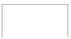 | 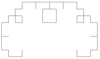 |
| Gosper Curve Level 1 | Gosper Curve Level 2 | Gosper Curve Level 6 |
| Reading: Before going further, you should have finished reading all of SICP, Chapter 1 and GEB, Chapter 5. |
|
Downloads: You will need to download this file to your machine: curve.ss
Create a new definitions file by selecting File | New. Put, (load "curve.ss") at the beginning of that file. This loads all the definitions from the curve.ss file. Edit your definitions after that. Click Save frequently to save your work (remember that Execute does not save your definitions). The first time you Save, DrScheme will ask you for a filename. Remember to make sure the Language is set to Full Scheme by selecting Language | Choose Language from the DrScheme menu. A dialog box will appear. Select Full Scheme in the Language choice menu and Graphical (MrEd) in the right radio box. |
Drawing Points
A curve is a (possibly infinite) set of points. We can draw a curve by mapping points on the curve to pixels on the screen.
For this assignment, we will use a coordinate system from (0, 0) to (1, 1):
| (0.0, 1.0) | (1.0, 1.0) | ||
|
| |||
| (0.0, 0.0) | (1.0, 0.0) |
Points have x and y coordinates. To represent points we would like to define functions make-point, x-of-point and y-of-point such that:
> (x-of-point (make-point 0.2 0.4))
0.2

> (y-of-point (make-point 0.2 0.4))
0.4
Here's one way:
(define (make-point x y)
   (lambda (selector) (if selector x y)))

(define (x-of-point point) (point #t))
(define (y-of-point point) (point #f))
The function make-point takes two parameters and returns a function. The returned function is a function of one parameter, selector. If the parameter is false (#f), it returns the y parameter; otherwise it returns the x parameter.
We have provided two procedures for drawing on the window in curve.ss:
- (window-draw-point point) — Draw a black dot on the window at the point point. For example, (window-draw-point (make-point 0.5 0.5)) will place a black dot in the center of the window. (The point is only one pixel, so it is hard to see.)
- (window-draw-line point0 point1) — Draw a
black line from point0 to point1. For example,
(window-draw-line (make-point 0.0 0.0) (make-point 1.0 1.0)) will
draw a diagonal line from the bottom left corner to the top right
corner.
- (graphics-clear) — Clear the graphics window.
| Question 1: Define a function that uses make-point, window-draw-point and window-draw-line to draw a simple picture of a boat. The primary point of this not particularly pointed problem, is to point out how to practice producing pictures by putting point procedures in proximity pointedly. (That is, there is nothing to turn in for this, but attempt the next question until you can do this.) |
Curves
Building upon points, we can make curves and lines (straight lines are just a special kind of curve). We can think of curves as functions from values to points. One way to represent a curve is as a function that evaluates to a point for every value between 0.0 and 1.0. For instance,(define (mid-line t) (make-point t 0.5))defines a curve that is a horizontal line across the middle of the window. If we apply mid-line to a value x, we get the point (x, 0.5). Hence, if we apply mid-line to all values between 0.0 and 1.0, we get a horizontal line.
Predict what (x-of-point (mid-line 0.7)) and (y-of-point (mid-line 0.7)) evaluate to. Try them in your Interactions window.
Of course, there are infinitely many values between 0.0 and 1.0, so we can't apply it to all of them. Instead, we select enough values to show the curve well. To draw a curve, we need to apply the curve function to many values in the range from 0.0 to 1.0 and draw each point it evaluates to. Here's a function that does that:
(define (draw-curve-points curve n)
  (define (worker t step)
    (if (<= t 1.0)
        (begin
          (window-draw-point (curve t))
          (worker (+ t step) step))))
  (worker 0.0 (/ 1 n)))
The function draw-curve-points takes a function representing
a curve, and n, the number of points to draw. The inner
function, worker is defined recursively: if
t is less than or equal to 1.0, we draw the current point using
(window-draw-point (curve t)) and draw the rest of the points
by evaluating (worker curve (+ t step)
step)). The code uses the special form begin. The
evaluation rule for begin is:
Evaluation Rule 4-begin. To evaluate (begin Expression1 Expression2 ... Expressionk), evaluate each sub-expression in order from left to right. The value of the begin expression is the value of Expressionk.We stop once t is greater than 1.0, since we defined the curve over the interval [0.0, 1.0].
A similar function, draw-curve-connected draw a curve by making a line between each point on the curve and the next point. Think about how you would define draw-curve-connected. (You can see how we defined it in the provided code.)
Question 2:
|
The good thing about defining curves using functions, is it is easy to modify and combine then in interesting ways.
For example, the function rotate-ccw takes a curve and rotates it 90 degrees counter-clockwise. It just swaps the x and y points:
(define (rotate-ccw curve)
  (lambda (t)
    (make-point
     (- (y-of-point (curve t)))
     (x-of-point (curve t)))))
The function rotate-ccw is a function that takes a function (a curve) and returns a function that is a curve. Predict what (draw-curve-points (rotate-ccw mid-line) 1000) will do before trying it in your Interactions window.
Here's another example:
(define (shrink curve scale)
  (lambda (t)
    (make-point
     (* scale (x-of-point (curve t)))
     (* scale (y-of-point (curve t))))))
Try to predict what (draw-curve-points (shrink mid-line .5)
1000) will do before trying it in your Interactions window.
The shrink doesn't produce quite what we want because in addition to changing the size of the curve, it moves it around. Make sure you understand why this happens.
One way to fix this problem is to center our curves around (0, 0) and then translate them to the middle of the screen. We can do this by adding or subtracting constants to the points they produce:
(define (translate curve x y)
  (lambda (t)
    (make-point
     (+ x (x-of-point (curve t)))
     (+ y (y-of-point (curve t))))))
Now we have translate, it makes more sense to define
mid-line this way:
(define (horiz-line t)
   (make-point t 0))

(define mid-line (translate horiz-line 0 0.5))
To check you understand everything so far, use translate, horiz-line and shrink to draw a line half the width of the window centered in the middle of the display window.
In addition to alterning the points a curve produces, we can alter a curve by changing the t values it will see. For example,
(define (first-half curve)
   (lambda (t)
      (curve (/ t 2))))
Is a function that takes a curve, and produces a new curve that is just
the first half of the passed curve.
Predict what (draw-curve-points (first-half mid-line) 1000) will do. Then try it in your Interactions window to check you were right. Predict what (draw-curve-points (first-half (first-half mid-line)) 1000)) will do. Then try it in your Interactions window to check you were right. (Remember to use (graphics-clear) to clear the screen so you can see the new curve without the old one.)
Since the curve is a parameter, we can use draw-curve-points to draw any curve just by passing in a different function. For example, if we remember geometry well (don't worry, you don't have to for this assignment) we can draw a circle using:
(define (unit-circle t)
    (make-point (sin (* 2pi t)) (cos (* 2pi t))))
This makes a circle of radius 1, centered at (0, 0). Since our
window only shows the coordinate space from (0.0, 0.0) to
(1.0, 1.0) most of the circle will not be visible.
Try to predict what (draw-curve-points unit-circle 1000) does, and then try it in your Interactions window. Note that draw-curve-points prints out a warning message every time it tries to draw a point that does not fit in the display window. These warnings may be helpful when you try to draw a curve but don't see anything on the display.
To make a circle that fits on the display, we need to shrink it and translate it so the center of the circle is in the middle of the display — (0.5, 0.5). Here's how: (draw-curve-points (translate (shrink unit-circle .25) 0.5 0.5) 1000)
|
Question 3: Define a function that draws a smiley face. You will probably need to
define a function similar to first-half, but that takes less
than half of the curve. You shouldn't need to use any fancy geometry
(e.g., sin or cos), but instead use functions to alter
the center-circle curve we have already defined to make the
smile, eyes and nose. If you don't like procedures yet, you can draw a
frowny face instead. If you are having a hard time drawing the mouth,
read ahead a bit in the problem set (but try to do this with your own
code).
Turn in the code you defined and a print out of your display window. To print out the graphics window:
|
Composing Functions
To draw your smiley face, you probably did something like:
  (draw-curve-points
   (translate
    (rotate-ccw (flip-vertically (first-half (shrink unit-circle .25))))
    0.5 0.5)
   1000)
This composes lots of functions together to turn a radius on circle
(the curve produced by unit-circle) into a small half-circle
oriented like a smile and centered in the display window.
One of the steps was to flip-vertically and rotate-ccw to turn the curve 270 degrees counter-clockwise (or 90 degrees clockwise). We can define a function that does this:
(define (rotate-cw curve)
   (rotate-ccw (flip-vertically curve)))
Composing functions is a common task. We can define a compose function that composes two functions:
(define (compose f g)
   (lambda (x) (f (g x))))
Then we can define rotate-cw as:
(define rotate-cw (compose rotate-ccw flip-vertically))
Question 4:
If you aren't quite so happy about procedures, you may want to make a
smiley face with a smaller smile. You could do that by applying
first-half twice to get a quarter-curve (this produces a
lop-sided smile, but that's okay)
:
      (draw-curve-points
       (translate (rotate-cw (first-half (first-half (shrink unit-circle .25)))) 0.5 0.5)
       1000)
|
Hint: Your function will look like this (the parts in < ... > brackets are what you need to fill in):
(define (n-times f n)
   (if (= n 1)
       f         ; One time, is just f
       (compose <fill this in>
                (n-times f <fill this in>))))
Once you've defined n-times, you should be able to use this
code to draw a very small and lopsided smiley:
(draw-curve-points
 (translate (rotate-cw
             ((n-times first-half 4)
              (shrink unit-circle .25)))
            0.5 0.5)
 1000)
Note that (n-times first-half 4) evaluates to a function.
That's why there are two (('s before the n-times —
we need to apply the function resulting from (n-times first-half
4) to the function resulting from (shrink unit-circle .25).
Curve Transforms
The provided code includes several other functions that transform curves including:- scale-x-y curve x-scale y-scale - stretches a curve along the x and y axis by using the scale factors given
- scale curve scale - stretches a curve along the x and y axis by using the same scale factor
- rotate-around-origin curve degrees - will take a curve and rotate it counterclockwise by a given number of degrees.
It is also useful to have curve transforms where curves may be combined. We call a transformation where two curves are used to produce a new curve a binary transformation.
connect-rigidly is a simple type of binary transform. The function will return a curve which consists of curve1 followed by curve2. The starting point of the new curve is the starting point of curve1 and the end point of curve2 is the ending point of the new curve.
(define (connect-rigidly curve1 curve2)
    (lambda (t)
      (if (< t (/ 1 2))
          (curve1 (* 2 t))
          (curve2 (- (* 2 t) 1)))))
Predict what (draw-curve-points (connect-rigidly vertical-mid-line
mid-line) 1000) will do. Is there any difference between that
and (draw-curve-points (connect-rigidly mid-line
vertical-mid-line) 1000)? Check your predictions in the
Interactions window.
|
Question 5:
Define a new smiley drawing function, smiley-curve but this time make it a single curve. The same smiley face you drew in Question 3 should now appear when you do, (draw-curve-points smiley-curve 1000)Some parts of your smiley face probably appear dotty (instead of as solid lines). Explain why some parts of your smiley face are more dotty than others. Optional (bonus points - don't try this until you have finished the rest of the problem set). Define a better function for turning many curves into a single curve that does not have this problem. |
Gosper Curves
If you look back at the beginning of the problem set, you can see three
example iterations of the Gosper Curve. The curve starts off as a
straight line at level 0, then transforms into what is pictured at
level 1. After level 1, the curve from one iteration to the next will
rotate the previous iteration and translate it 50% to the right and
50% of the viewport up. This is to ensure that the second curve’s
beginning will coincide with the first curve’s endpoint. Putting this
set of steps together brings us to the curve transformation function
gosperize:
(define (gosperize curve)
  (let ((scaled-curve (scale-x-y curve
                                 (/ (sqrt 2) 2) (/ (sqrt 2) 2))))
    (connect-rigidly (rotate-around-origin scaled-curve (/ pi 4))
                     (translate
                      (rotate-around-origin scaled-curve (/ -pi 4))
                      .5 .5))))
Building upon this, we can repeatedly call this function dependent on
the number of iterations, or levels, we want to see using the
n-times function you defined in Question 4:
(define (gosper-curve level)
    ((n-times gosperize level) unit-line))
Finally, to actually see all this in action we have a drawing function for gosper curves:
(define (show-connected-gosper level)
  (draw-curve-connected
   (squeeze-rectangular-portion (gosper-curve level) -.5 1.5 -.5 1.5)
   1000))
The squeeze-rectangluar-portion translates and scales a curve to show the part in the region specified by the parameters (-.5, 1.5), (-.5, 1.5).
| Question 6: Draw some gosper curves using (show-connected-gosper level). Print out your graphics window. Note that if all the code you wrote earlier works correctly, there is no new code required for this. |
Efficiency
Our implementation is really slow. One of the reasons for this is many of our curve transformations have to evaluate (curve t) more than once. For example, scale-x-y evaluates (curve t) twice:
(define (scale-x-y curve x-scale y-scale)
  (lambda (t)
    (make-point (* x-scale (x-of-point (curve t)))
                (* y-scale (y-of-point (curve t))))))
We can make a more efficient version of scale-x-y by only evaluating (curve t) once:
(define (scale-x-y curve x-scale y-scale)
  (lambda (t)
    (let ((ct (curve t)))
      (make-point (* x-scale (x-of-point ct))
                  (* y-scale (y-of-point ct))))))
The let construction is a short cut for:
(define (scale-x-y curve x-scale y-scale)
  (lambda (t)
    ((lambda (ct)
       (make-point (* x-scale (x-of-point ct))
                   (* y-scale (y-of-point ct))))
     (curve t))))
Question 7:
|
Enhancements
Everything below here is optional. You may receive a some bonus points for especially good answers and may get a poster of any particularly nice fractals, but you are not required or expected to do anything more. This section provides some suggestions for interesting things you might do to make more interesting fractals, but you are encouraged to come up with your own ideas for doing interesting things with curves.Other Curves. The gosperize procedure takes a curve parameter, so we can gosperize more interesting curves than the unit-line. Try gosperizing some other curves to make an interesting picture. Try gosperizing the smiley-curve you produced in Question 5. The result is an approximation of what CS200 students would look like if they wait until the night before it is due to start Problem Set 3.
Other Angles. The gosper curves we’ve been working with have had the angle of rotation fixed at 45 degrees. To draw more varied Gosper curves, try defining a (gosperize-angle curve angle) function where the angle to turn is a parameter.
Color. Our curves are plain black lines. A more interesting fractal would use color also. Try modifying the definition of make-point, so that points have color in addition to x and y coordinates. You will need to change many of the other functions also, since make-point will now take an extra parameter giving the color of the point. Try to define a colorful version of gosperize.
| Credits: This problem set was adapted for UVA CS 200 Spring 2002 from MIT 6.001 Problem Set 2 from Fall 1996 by Dante Guanlao and David Evans and tested by Stephen Liang. |
