| Problem Set 2: Function Fractals |
Out: 22 January 2003 Due: Monday, 3 February 2003, beginning of class |
Collaboration Policy - Read Carefully
For this problem set, you are required to work with your pseudo-randomly assigned partner listed below. You and your partner should turn in one assignment with both of your names on it. You should read the whole problem set yourself and think about the questions before beginning to work on them with your partner (listed below).
In addition to your partner, you may discuss this assignment with other students in the class and ask and provide help in useful ways. You may consult any outside resources you wish including books, papers, web sites and people except for materials from last year's CS200 course. If you use resources other than the class materials, indicate what you used along with your answer.
| Arielle Myhre (aam3m@virginia.edu) Nolan Madge (nrm5z@virginia.edu) |
Andrew Connors (apc7a@virginia.edu) Jerome McGann (jjm2f@virginia.edu) |
David Madaras (dmm3j@virginia.edu) Andrea Jacobs (amj2d@virginia.edu) |
Daniel Greene (dpg7g@virginia.edu) Mai Hong Pham (mhp3b@virginia.edu) |
| Edward Mitchell
(ejm5p@virginia.edu) Robert Schweizer (rts4j@virginia.edu) |
Grace Chang (gjc5h@virginia.edu) Sarah Payne (srp2e@virginia.edu) |
Jessica Nute (jln2f@virginia.edu) Margaret Olson (molson@virginia.edu) |
Jessica Ruge (jmr9z@virginia.edu) Katrina Salmons (ks2wf@virginia.edu) |
| Krystal Ball (kmb6j@virginia.edu) Matthew Mehalso (mm4md@virginia.edu) |
Lauren Cryan (lac4z@virginia.edu) Anoop Gambhir (asg4y@virginia.edu) |
Lindy Brown
(lcb4b@virginia.edu) Mary Eckerle (mke4b@virginia.edu) |
Owen Jones (ofj4f@virginia.edu)
Patrick Lane (plane@virginia.edu) |
| Patrick Rooney (pjr2y@virginia.edu) Sean Mays (sdm8s@virginia.edu) |
Steven Marchette (sam7p@virginia.edu) Hassan Tahir (hassan@tahirs.com) |
Samuel Sangobowale (sos8v@virginia.edu) Qi Wang (qw2d@virginia.edu) |
Sarah Bergkuist (srb5z@virginia.edu) Salvatore Guarnieri (sg8u@virginia.edu) |
| Timothy Shull (ts8b@virginia.edu) James Lee (jl6eu@virginia.edu) |
Victoria Lynch (vnl9w@virginia.edu) Ramsey Arnaoot (rma3n@virginia.edu) |
William Brand (wtb2f@virginia.edu) Justin Alexander Pan (jap4u@virginia.edu) |
Zachary Hill (zfh3e@virginia.edu) Chalermpong Worawannotai (cw7r@virginia.edu) |
Purpose
- Become comfortable with procedures as parameters and results.
- Get some practice defining recursive procedures.
- Play (nicely) with fractals.
Unlike in Problem Set 1, you are expected to be able to understand
all the code provided for this problem set (and all future
problem sets in this class unless specifically explained otherwise).
This problem set requires less reading and introduces fewer new ideas
than Problem Set 1, but expects you to write a lot more code. As
always, we recommend you start early and take advantage of
these staffed lab hours:
Thursday, 23 January, 8-9pm (Rachel) |
Background
The name "fractal" was invented by Benoit Mandlebrot from the Latin adtive fractus, meaning to break (as in fracture). A fractal is a geometric shape that can be recursively broken down into smaller parts. Unlike a mosaic, the smaller parts of a fractal all look like the original shape, just scaled down. There are many fractal-like structures found in the real world including clouds, coastlines, trees and stock market fluctuations.
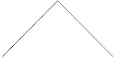
Fractals receive a lot of attention because of their interesting mathematical properties, but also because they look really cool. There are several types of fractals but the fractal we will be working with in this assignment is the Gosper Curve (you'll see a few more in PS3), pictures created by the repetition of a simple process. At every iteration of the Gosper curve, an approximation to the fractal curve is made. The next iteration consists of two scaled-down copies of the current iteration, now rotated 45 degrees and connected end to end.
 |
 | 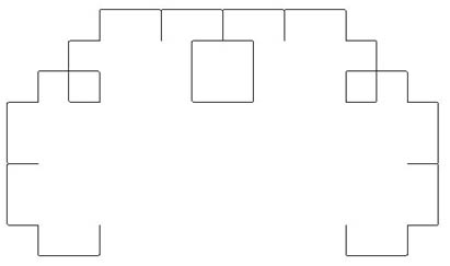 |
| Gosper Curve Level 1 | Gosper Curve Level 2 | Gosper Curve Level 6 |
| Reading: Before going further, you should have finished reading all of SICP, Chapter 1 and GEB, Chapter 5. |
|
Download: Download ps2.zip
to your machine and unzip it into your home directory
J:\cs200\ps2.
This file contains: Remember to click Save frequently to save your work (remember that Execute does not save your definitions) and make sure the language is set to Pretty Big (includes MrEd and Advanced from the PLT menu. |
Drawing Points
A curve is a (possibly infinite) set of points. We can draw a curve by mapping points on the curve to pixels on the screen. For this assignment, we will use a Cartesian coordinate system from (0, 0) to (1, 1):
| (0.0, 1.0) | (1.0, 1.0) | ||
|
| |||
| (0.0, 0.0) | (1.0, 0.0) |
We can describe the location of a point using its horizontal and vertical location given by x and y coordinates. To represent points we would like to define functions make-point, x-of-point and y-of-point that behave like this:
Here's one way:> (x-of-point (make-point 0.2 0.4))
0.2
> (y-of-point (make-point 0.2 0.4))
0.4
(define (make-point x y)
   (lambda (selector) (if selector x y)))

(define (x-of-point point) (point #t))
(define (y-of-point point) (point #f))
The function make-point takes two parameters and returns a function. The returned function is a function of one parameter, selector. If this parameter is false (#f), it returns the y parameter of make-point; otherwise it returns the x parameter of make-point.
We have provided two procedures for drawing on the window in curve.ss:
- (window-draw-point point)
— Draw a black dot on the window at the point point. For
example,
(window-draw-point (make-point 0.5 0.5))
will place a black dot in the center of the window. (The point is only one pixel, so it is hard to see.) - (window-draw-line point0 point1) — Draw a
black line from point0 to point1. For example,
(window-draw-line (make-point 0.0 0.0) (make-point 1.0 1.0))
will draw a diagonal line from the bottom left corner to the top right corner.
| Question 1: Define a procedure that uses make-point, window-draw-point and window-draw-line to draw a simple picture of a boat. (You don't need to turn in your boat picture unless it is especially interesting.) |
Curves
Building upon points, we can make curves and lines (straight lines are just a special kind of curve). We can think of curves as functions that take us from values to points. One way to represent a curve is as a function that evaluates to a point for every value between 0.0 and 1.0. For instance,(define (mid-line t) (make-point t 0.5))
defines a curve that is a horizontal line across the middle of the window. If we apply mid-line to a value x, we get the point (x, 0.5). Hence, if we apply mid-line to all values between 0.0 and 1.0, we get a horizontal line.
Predict what each of these expressions evaluates to:
- (x-of-point (mid-line 0.7))
- (y-of-point (mid-line 0.7))
An ideal curve would result from applying our curve procedure to every value between 0.0 and 1.0. Of course, there are infinitely many values between 0.0 and 1.0, so we can't apply it to all of them. Instead, we select enough values to show he curve well. To draw a curve, we need to apply the curve function to many values in the range from 0.0 to 1.0 and draw each point it evaluates to. Here's a function that does that:
(define (draw-curve-points curve n)
  (define (worker t step)
    (if (<= t 1.0)
        (begin
          (window-draw-point (curve t))
          (worker (+ t step) step))))
  (worker 0.0 (/ 1 n)))
The function draw-curve-points takes a function representing
a curve, and n, the number of points to draw. The inner
function, worker is defined recursively: if
t is less than or equal to 1.0, we draw the current point using
(window-draw-point (curve t)) and draw the rest of the points
by evaluating (worker curve (+ t step)
step)). We use begin to evaluate two expressions inside
the if (check the begin evaluation rule).
A similar function, draw-curve-connected, draws a curve by making a line between each point on the curve and the next point. Think about how you would define draw-curve-connected. Once you have a good idea how to define it, look at the provided code in curve.ss to see if we defined it the same way.
Question 2:
|
The good thing about defining curves as functions is it is easy to modify and combine then in interesting ways.
For example, the function rotate-ccw takes a curve and rotates it 90 degrees counter-clockwise by swapping the x and y points:
(define (rotate-ccw curve)
  (lambda (t)
    (make-point
     (- (y-of-point (curve t)))
     (x-of-point (curve t)))))
Note that (rotate-ccw c) evaluates to a curve! The function rotate-ccw is a function that takes a function (a curve) and returns a function that is a curve.
Predict what (draw-curve-points (rotate-ccw mid-line) 1000) will do. Confirm your prediction by trying it in your Interactions window.
Here's another example:
(define (shrink curve scale)
  (lambda (t)
    (make-point
     (* scale (x-of-point (curve t)))
     (* scale (y-of-point (curve t))))))
Predict what (draw-curve-points (shrink mid-line .5)
1000) will do, and then try it in your Interactions window.
The shrink procedure doesn't produce quite what we want because in addition to changing the size of the curve, it moves it around. Make sure you understand why this happens. Try shrinking a few different curves to make sure.
One way to fix this problem is to center our curves around (0,0) and then translate them to the middle of the screen. We can do this by adding or subtracting constants to the points they produce:
(define (translate curve x y)
  (lambda (t)
    (make-point (+ x (x-of-point (curve t))) (+ y (y-of-point (curve t))))))
Now we have translate, it makes more sense to define
mid-line this way:
(define (horiz-line t) (make-point t 0))
(define mid-line (translate horiz-line 0 0.5))
To check you understand everything so far, use translate, horiz-line and shrink to draw a line half the width of the window that is centered in the middle of the display window.
In addition to altering the points a curve produces, we can alter a curve by changing the t values it will see. For example,
(define (first-half curve)
   (lambda (t) (curve (/ t 2))))
is a function that takes a curve and produces a new curve that is just the first half of the passed curve.
Predict what each of these expressions will do:
- (draw-curve-points (first-half mid-line) 1000)
- (draw-curve-points (first-half (first-half mid-line)) 1000))
Since the curve is a parameter, we can use draw-curve-points to draw any curve just by passing in a different function. For example, if we remember geometry well (don't worry, you don't have to remember any geometry yourself for this assignment) we can draw a circle using:
(define (unit-circle t)
    (make-point (sin (* 2pi t)) (cos (* 2pi t))))
This makes a circle of radius 1, centered at (0, 0). Since our
window only shows the coordinate space from (0.0, 0.0) to
(1.0, 1.0) most of the circle will not be visible.
Try to predict what (draw-curve-points unit-circle 1000) does, and then try it in your Interactions window. Note that draw-curve-points prints out a warning message every time it tries to draw a point that does not fit in the display window. These warnings may be helpful when you try to draw a curve but don't see anything on the display.
To make a circle that fits on the display, we need to shrink it and translate it so the center of the circle is in the middle of the display: (0.5, 0.5). Here's how: (draw-curve-points (translate (shrink unit-circle .25) 0.5 0.5) 1000)
|
Question 3: Define a function that draws a smiley face. To make
the mouth, you may need to define a function similar to
first-half, but that takes less than half of the curve. You
shouldn't need to use any fancy geometry (e.g., sin or
cos), but instead use functions to alter the
center-circle curve we have already defined to make the mouth,
eyes and nose. If you don't like procedures yet, you can draw a frowny
face instead (but the eyes must be open!). If you are having a hard
time drawing the mouth, read ahead a bit in the problem set (but try to
do this with your own code first).
Turn in the code you defined and a print out of your display window (see directions following). |
To print out the graphics window:
- Drag your display window so that it's near the left edge of the screen (this will make things a bit easier)
- Press the PrtScn (or PrintScrn) key (above the Insert key on most keyboards). This will take a snapshot of your screen and save it to the Windows Clipboard.
- Open MS Paint (Start | Accessories | Paint) and press Ctrl-V to paste your screenshot. (Select "Yes" if it asks you whether you want to enlarge the bitmap if your screenshot is bigger than the default bitmap size.)
- Select File | Print, and print page 1 only — your display window should fit into the portion that is printed. (Ask for help if it doesn't come out right.)
Composing Functions
To draw your smiley face, you probably did something like:
  (draw-curve-points
    (translate
     (rotate-ccw
      (flip-vertically (first-half (shrink unit-circle .25))))
     0.5 0.5)
    1000)
This composes lots of functions together to turn a unit radius circle
(the curve produced by unit-circle) into a small half-circle
oriented like a smile and centered in the display window.
One of the steps was to flip-vertically and rotate-ccw to turn the curve 270 degrees counter-clockwise (or 90 degrees clockwise). We can define a function that does this by composing rotate-ccw and flip-vertically:
(define (rotate-cw curve)
   (rotate-ccw (flip-vertically curve)))
Composing functions is a common task. We can define a compose function that composes two functions (each of which must take a single parameter):
(define (compose f g)
   (lambda (x) (f (g x))))
Then we can define rotate-cw as:
(define rotate-cw (compose rotate-ccw flip-vertically))
Question 4:
If you aren't quite so happy about procedures, you may want to make a
smiley face with a smaller smile. You could do that by applying
first-half twice to get a quarter-curve (this produces a
lop-sided smile, but that's okay):
   (draw-curve-points
    (translate
     (rotate-cw
      (first-half (first-half (shrink unit-circle .25))))
     0.5 0.5)
    1000)
|
Hint: Your function will look like this (the parts in < ... > brackets are what you need to fill in):
(define (n-times f n)
   (if (= n 1)
       f         ; One time, is just f
       (compose <fill this in>
                (n-times f <fill this in>))))
Once you've defined n-times, you should be able to use this
code to draw a very small and lopsided smiley:
(draw-curve-points
 (translate (rotate-cw
             ((n-times first-half 4)
              (shrink unit-circle .25)))
            0.5 0.5)
 1000)
Note that (n-times first-half 4) evaluates to a function.
That's why there are two (('s before the n-times —
we need to apply the function resulting from (n-times first-half
4) to the function resulting from (shrink unit-circle .25).
Curve Transforms
The provided code includes several other functions that transform curves including:- (scale-x-y curve x-scale y-scale) — evalutes to curve stretched along the x and y axis by using the scale factors given
- (scale curve scale) — evaluates to curve stretched along the x and y axis by using the same scale factor
- (rotate-around-origin curve degrees) — evaluates to curve rotated counterclockwise by the given number of degrees.
It is also useful to have curve transforms where curves may be combined. An example is (connect-rigidly curve1 curve2) which evaluates to a curve that consists of curve1 followed by curve2. The starting point of the new curve is the starting point of curve1 and the end point of curve2 is the ending point of the new curve. Here's how connect-rigidly is defined:
(define (connect-rigidly curve1 curve2)
    (lambda (t)
      (if (< t (/ 1 2))
          (curve1 (* 2 t))
          (curve2 (- (* 2 t) 1)))))
Predict what (draw-curve-points (connect-rigidly vertical-mid-line
mid-line) 1000) will do. Is there any difference between that
and (draw-curve-points (connect-rigidly mid-line
vertical-mid-line) 1000)? Check your predictions in the
Interactions window.
|
Question 5:
|
Gosper Curves
The beginning of this problem set shows three example iterations of
the Gosper Curve. The curve starts off as a straight line at level 0,
then transforms into what is pictured at level 1. After level 1, the
curve from one iteration to the next will rotate the previous
iteration and translate it 50% to the right and 50% of the viewport
up. This is to ensure that the second curve's beginning will coincide
with the first curve's endpoint. Putting these steps together gives
us the curve transformation function gosperize:
(define (gosperize curve)
  (let ((scaled-curve (scale-x-y curve (/ (sqrt 2) 2) (/ (sqrt 2) 2))))
    (connect-rigidly (rotate-around-origin scaled-curve (/ pi 4))
                     (translate (rotate-around-origin scaled-curve (/ -pi 4)) .5 .5))))
Building upon this, we can repeatedly call this function dependent on
the number of iterations, or levels, we want to see using the
n-times function you defined in Question 4:
(define (gosper-curve level)
    ((n-times gosperize level) unit-line))
Finally, to actually see all this in action we have a drawing function for gosper curves:
(define (show-connected-gosper level)
  (draw-curve-connected
   (squeeze-rectangular-portion (gosper-curve level) -.5 1.5 -.5 1.5)
   1000))
The squeeze-rectangluar-portion translates and scales a curve to show the part in the region specified by the parameters (-.5, 1.5), (-.5, 1.5).
Draw some gosper curves using (show-connected-gosper level). Note that if all the code you wrote earlier works correctly, there is no new code required for this.
Efficiency
Our implementation is really slow. One of the reasons for this is many of our curve transformations have to evaluate (curve t) more than once. For example, scale-x-y evaluates (curve t) twice:
(define (scale-x-y curve x-scale y-scale)
  (lambda (t)
    (make-point (* x-scale (x-of-point (curve t)))
                (* y-scale (y-of-point (curve t))))))
We can make a more efficient version of scale-x-y by only evaluating (curve t) once:
(define (scale-x-y curve x-scale y-scale)
  (lambda (t)
    (let ((ct (curve t)))
      (make-point (* x-scale (x-of-point ct))
                  (* y-scale (y-of-point ct))))))
The let construction is a short cut for:
(define (scale-x-y curve x-scale y-scale)
  (lambda (t)
    ((lambda (ct)
       (make-point (* x-scale (x-of-point ct))
                   (* y-scale (y-of-point ct))))
     (curve t))))
Question 6:
|
You are encouraged to answer these questions by thinking about what the code does. You can use the trace procedure to observe applications of a procedure in an evaluation. For example, if you evaluate (trace unit-line), then everytime unit-line is applied, DrScheme will print out tracing information showing the application. (Don't try counting the number of applications from (gosper-curve 5) by hand!)
Optional Enhancements
Everything below here is optional. You may receive a some bonus points for especially good answers and any particularly nice fractals will be posted on the course web site, but you are not required or expected to do anything more. This section provides some suggestions for interesting things you might do to make more interesting fractals, but you are encouraged to come up with your own ideas for doing interesting things with curves.Other Curves. The gosperize procedure takes a curve parameter, so we can gosperize more interesting curves than the unit-line. Try gosperizing some other curves to make an interesting picture. Try gosperizing the smiley-curve you produced in Question 5. The result is an approximation of what CS200 students would look like if they wait until the night before it is due to start Problem Set 3.
Other Angles. The gosper curves we've been working with have had the angle of rotation fixed at 45 degrees. To draw more varied Gosper curves, try defining a (gosperize-angle curve angle) function where the angle to turn is a parameter.
Color. Our curves are plain black lines. A more interesting fractal would use color also. Try modifying the definition of make-point so that points have color in addition to x and y coordinates. You will need to change many of the other functions also, since make-point will now take an extra parameter giving the color of the point. Try to define a colorful version of gosperize.
| Credits: This problem set was revised for UVA CS200 Spring 2003 by Rachel Dada and David Evans. The original version for UVA CS 200 Spring 2002 was adapted from MIT 6.001 Problem Set 2 from Fall 1996 by Dante Guanlao and David Evans and tested by Stephen Liang. |
