CS200: Problem Set 3: List Fractals

University of Virginia, Department of Computer Science
CS200: Computer Science, Spring 2003

Problem Set 3: L-System Fractals Out: 3 February 2002
Due: 12 February 2002, before class

Collaboration Policy - Read Carefully
For this problem set, you are required to work with your assigned partner listed below. Partners were assigned based (loosely) on your answers to the registration survey question 12. You and your partner should turn in one assignment with both of your names on it. You should read the whole problem set yourself and think about the questions before beginning to work on them with your partner (listed below).
In addition to your partner, you may discuss this assignment with other students in the class and ask and provide help in useful ways. You may consult any outside resources you wish including books, papers, web sites and people except for materials from last year's CS200 course. If you use resources other than the class materials, indicate what you used along with your answer.

Andrea Jacobs (amj2d@virginia.edu)
Lauren Cryan (lac4z@virginia.edu) Andrew Connors (apc7a@virginia.edu)
Nolan Madge (nrm5z@virginia.edu) Anoop Gambhir (asg4y@virginia.edu)
Zachary Hill (zfh3e@virginia.edu)
Chalermpong Worawannotai (cw7r@virginia.edu)
Sarah Bergkuist (srb5z@virginia.edu) Jerome McGann (jjm2f@virginia.edu)
Jessica Nute (jln2f@virginia.edu) Jessica Ruge (jmr9z@virginia.edu)
James Lee (jl6eu@virginia.edu)
Justin Pan (jap4u@virginia.edu)
Grace Chang (gjc5h@virginia.edu) Krystal Ball (kmb6j@virginia.edu)
David Madaras (dmm3j@virginia.edu) Lindy Brown (lcb4b@virginia.edu)
Matthew Mehalso (mm4md@virginia.edu)
Margaret Olson (molson@virginia.edu)
Edward Mitchell (ejm5p@virginia.edu) Mary Eckerle (mke4b@virginia.edu)
Arielle Myhre (aam3m@virginia.edu) Patrick Lane (plane@virginia.edu)
Katrina Salmons (ks2wf@virginia.edu)
Patrick Rooney (pjr2y@virginia.edu)
Jeffrey Arrington (jda7d@virginia.edu) Ramsey Arnaoot (rma3n@virginia.edu)
Qi Wang (qw2d@virginia.edu) Salvatore Guarnieri (sg8u@virginia.edu)
Sarah Payne (srp2e@virginia.edu)
Samuel Sangobowale (sos8v@virginia.edu)
Sean Mays (sdm8s@virginia.edu) Timothy Shull (ts8b@virginia.edu)
Steven Marchette (sam7p@virginia.edu) William Brand (wtb2f@virginia.edu)
Daniel Greene (dpg7g@virginia.edu)

This problem set is harder than Problem Set 2. We recommend you start early and take advantage of these staffed lab hours:
Tuesday, 4 February: 8-9pm (Jacques)
Thursday, 6 February: 7-8pm (Spencer)
Thursday, 6 February: 8-9:30pm (Jacques)
Saturday, 8 February: 2-3:30pm (Spencer)
Sunday, 9 February: 8-9:30pm (Jacques)
Monday, 10 February: 6-7:30pm (Spencer)

Purpose

Get more practice with recursive definitions and procedures
Explore the power of rewrite rules
Learn to use lists
Write recursive functions that manipulate lists
Introduce data abstraction
Make some better fractals than you could in PS2

Reading: Before doing this problem set, you should read SICP 2.1 and 2.2 (you may skip section 2.2.4).

Download: Download ps3.zip to your machine and unzip it into your home directory J:\cs200\ps3.
This file contains:

ps3.ss — A template for your answers. You should do the problem set by editing this file.
curve-ps3.ss — Scheme code for drawing curves. This is similar to curve.ss from PS2, except we have made some improvements (as described later) that will help you draw better L-System Fractals.
lsystem.ss — provided incomplete code for producing L-System Fractals

Background

In Problem Set 2, you created fractals by manipulating procedures that represented curves. In this problem set, you will explore a different way of creating fractals known as the Lindenmayer system (or L-system). Aristid Lindemayer, a theoretical biologist at the University of Utrecht, developed the L-system in 1968 as a mathematical theory of plant development. In the late 1980s, he collaborated with Przemyslaw Prusinkiewicz, a computer scientist at the University of Regina, to explore computational properties of the L-system and developed many of the ideas on which this problem set is based.
The idea behind L-system fractals is that we can describe a curve as a list of lines and turns, and create new curves by rewriting old curves. Everything in an L-system curve is either a forward line (denoted by F), or a right turn (denoted by Ra where a is an angle in degrees clockwise). We can denote left turns by using negative angles.
We create fractals by recursively replacing all forward lines in a curve list with the original curve list. Lindemayer found that many objects in nature could be described using regularly repeating patterns. For example, the way some tree branches sprout from a trunch can be described using the pattern:
F O(R30 F) F O(R-60 F) F.
This is interpreted as: the trunk goes up one unit distance, a branch sprouts at an angle 30 degrees to the trunk and grows for one unit. The O means an offshoot — we draw the curve in the following parentheses, and then return to where we started before the offshoot. The trunk grows another unit and now another branch, this time at -60 degrees relative to the trunk grows for one units. Finally the trunk grows for one more unit. The branches continue to sprout in this manner as they get smaller and smaller, and eventually we reach the leaves.
We can describe this process using replacement rules:
Start: (F)
Rule: F ::= (F O(R30 F) F O(R-60 F) F)
Here are the commands this produces after two iterations:
Iteration 0: (F)
Iteration 1: (F O(R30 F) F O(R-60 F) F)
Iteration 2: (F O(R30 F) F O(R-60 F) F O(R30 F O(R30 F) F O(R-60 F) F) F O(R30 F) F O(R-60 F) F O(R-60 F O(R30 F) F O(R-60 F) F) F O(R30 F) F O(R-60 F) F)

Here's what that looks like:

Iteration 0
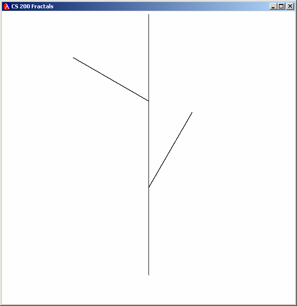Iteration 1
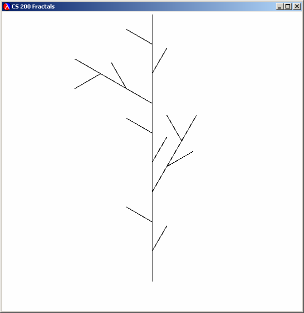Iteration 2

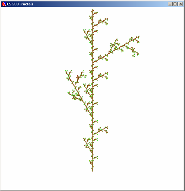Iteration 5
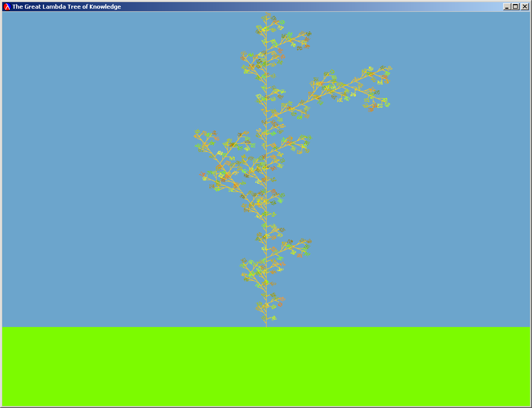The Great Lambda Tree of Infinite Knowledge and Ultimate Power

Note that L-system command rewriting is similar to the replacement rules in a BNF grammar. The important difference is that with L-system rewriting, each iteration replaces all instances of F in the initial string instead of just picking one to replace.
We can divide the problem of producing an L-system fractal into two main parts:

Produce a list of L-system commands that represents the fractal by rewriting according to the L-system rule; and
Drawing a list of L-system commands.
We will first work on producing the list of L-system commands, and then work on how to draw a list of L-system commands.

Representing L-System Commands

Here is a BNF grammar for L-system commands:

CommandSequence ::= ( CommandList )

CommandList ::= Command CommandList

CommandList ::=

Command ::= F

Command ::= RAngle

Command ::= OCommandSequence

Angle ::= Number

Question 1: Show that (F O(R-60 F) F) is a string in the language defined by our BNF grammar. To do this, you should start with CommandSequence, and show a sequence of replacements that follow the grammar rules that produce the target string. You can use the rule numbers above to identify the rules.

We need to find a way to turn strings in this grammar into objects we can manipulate in a Scheme program. We can do this by looking at the BNF grammar, and converting the non-terminals into Scheme objects.
;;; CommandSequence ::= ( CommandList )
(define make-lsystem-command list)

;;; We represent the different commands as pairs where the first item in the
;;; pair is a tag that indicates the type of command: 'f for forward, 'r for rotate
;;; and 'o for offshoot.  We use quoted letters to make tags, which evaluate to the
;;; letter after the quote.  The tag 'f is short for (quote f).

;;; Command ::= F
(define (make-forward-command) (cons 'f #f)) ;; No value, just use false.

;;; Command ::= RAngle
(define (make-rotate-command angle) (cons 'r angle))

;;; Command ::= OCommandSequence
(define (make-offshoot-command commandsequence) (cons 'o commandsequence))
Question 2: It will be useful to have procedures that take L-system commands as parameters, and return information about those commands. Define the following procedures in ps3.ss:

(is-forward? lcommand) — evaluates to #t if the parameter passed is a forward command (indicated by its first element being a 'f tag).
(is-rotate? lcommand)
(is-offshoot? lcommand)
(get-angle lcommand) — evaluates to the angle associated with a rotate command. Produces an error if the command is not a rotate command (see below for how to produce an error).
(get-offshoot-commands lcommand) — evaluates to the offshoot command list associated with an offshoot command. Produces an error if the command is not an offshoot command.

You will find the following procedures useful:

(car lst) — evaluates to the first element of the list parameter
(eq? v1 v2) — evaluates to #t if v1 and v2 are exactly the same; otherwise evaluates to false. For example, (eq? 's 's) evaluates to #t and (eq? 's 't) evaluates to #f.
(error message) — produces an error with message a string given as the first parameter. For example, (error "Yikes! Attempt to get-angle for a command that is not an angle command") would display the message in red and stop execution. It is useful to use error in your code so you will more easily identify bugs.
If you define these procedures correctly, you should produce these evaluations:

> (is-forward? (make-forward-command))

#t

> (is-forward? (make-rotate-command 90))

#f

> (get-angle (make-rotate-command 90))

90

> (get-angle (make-forward-command))

Yikes! Attempt to get-angle for a command that is not an angle command

You should be able to make up similar test cases yourself to make sure the other procedures you defined work.
Rewriting Curves
The power of the L-System commands comes from the rewriting mechanism. Recall how we described the tree fractal:
Start: (F)
Rule: F ::= (F O(R30 F) F O(R-60 F) F)

To produce levels of the tree fractal, we need a procedure that takes a list of L-system commands and replaces each F command with the list of L-system commands given by the rule.
So, for every command in the list:

If the command is an F command, replace it with the replacement commands
If the command is an RAngle command, keep it unchanged
If the command is an OCommandSequence command, recursively rewrite every command in the offshoot's command list the same way
One slight complication is that the replacement commands are a list of L-system commands, and we want to end up with a flat list of L-System commands.
For example, consider a simple L-System rewriting:
Start: (F)
Rule: F ::= (F R30 F)
We want to get:
Iteration1: (F R30 F)
Iteration2: (F R30 F R30 F R30 F)
but if we just replace F's with (F R30 F) lists, we would get:
Iteration1: ((F R30 F))
Iteration2: ((F R30 F) R30 (F R30 F))
The easiest way to fix this problem is to flatten the result. The code should look similar to many recursive list procedures you have seen (this code is provided in lsystem.ss):
(define (flatten-commands ll)
  (if (null? ll) ll
      (if (is-lsystem-command? (car ll))
	  (cons (car ll) (flatten-commands (cdr ll)))
	  (flat-append (car ll) (flatten-commands (cdr ll))))))

(define (flat-append lst ll)
  (if (null? lst) ll
      (cons (car lst) (flat-append (cdr lst) ll))))
Question 3: Define a procedure rewrite-lcommands in ps3.ss that takes a list of L-system commands as its first parameter. The second parameter is a list of L-system commands that should replace every forward command in the first list of commands in the result.
Here's the easy part:
(define (rewrite-lcommands lcommands replacement)
  (flatten-commands
   (map 
   ; Procedure to apply to each command
   lcommands)))
Complete the definition of rewrite-lcommands.
To make interesting L-system curves, we will need to apply rewrite-lcommands many times. We will leave that until the last question. First, we will work on turning sequences of L-system commands into curves we can draw.
Improving Our Curve Drawing
To help you draw better L-system Curves, we have provided a new version of the curve drawing code from PS2. You don't need to modify this code, but should understand the changes described below.

Points
In PS2, we represented points using a procedure:
(define (make-point x y)
   (lambda (selector) (if selector x y)))

(define (x-of-point point) (point #t))
(define (y-of-point point) (point #f))
Now that you know about lists, it is more natural to represent points using a cons pair:
(define (make-point x y) (cons x y))
(define (x-of-point point) (car point))
(define (y-of-point point) (cdr point))
Since we don't care too much about efficiency, we instead represent points using lists which will be slightly simpler:
(define (make-point x y) (list x y))
(define (x-of-point point) (car point))
(define (y-of-point point) (cadr point))
Note that we can change the way we represent points, and all the old PS2 code will still work without changing anything else (except it will run faster now). This is data abstraction, and is very important for building large programs.
Color
Our pictures will be more interesting if points can have color too. We represent a colored point using a list of three values: x, y and color:
(define (make-colored-point x y c) (list x y c))
(define (is-colored-point? point) (= (length point) 3))

;;; Regular points are black.  Colored points have a color.
(define (color-of-point point)
  (if (is-colored-point? point)
      (caddr point) 
      (make-color 0 0 0)))
We have defined colored points so the old colorless points still work (and appear black).
To make our curves appear in color, we need to change the way we draw points on the window to pass in the color also:
(define (window-draw-point point)
  ((draw-pixel window) (convert-to-position point) (color-of-point point)))
So that the color of our curves is not lost when we manipulate them, we also need to change all our curve-manipulating procedures to produce curves with the same colors as the original curve. For example, here is how we changed translate:
(define (translate curve x y)
  (lambda (t)
    (let ((ct (curve t)))
      (make-colored-point
       (+ x (x-of-point ct))
       (+ y (y-of-point ct))
       (color-of-point ct)))))
Distributing t Values
In PS2, when you drew the smiley curve, the t-values were not distributed evenly among all the curves in your smiley so the later curves appeared dotty. This wasn't too big a problem when only a few dozen curves were combined; we could just increase the number of points passed to draw-curve-points to have enough points to make a smooth curve. In this problem set, you will be drawing curves made up of thousands of connected curves. Just increasing the number of points won't help much, as you'll see in Question 4.
The way connect-rigidly was defined in PS2, we use all the t-values below 0.5 on the first curve, and use the t-values between 0.5 and 1.0 on the second curve:
(define (connect-rigidly curve1 curve2)
  (lambda (t)
      (if (< t (/ 1 2))
          (curve1 (* 2 t))
          (curve2 (- (* 2 t) 1)))))
If the second curve is the result of connecting two other curves, like (connect-rigidly c1 (connect-rigidly c2 c3)) then 50% of the points will be used to draw c1, 25% to draw c2 and 25% to draw c3.
Question 4: Define a procedure num-points that determines the approximate number of t-values that will be used for the n^th curve when drawing
   (connect-rigidly c1 (connect-rigidly c2 (connect-rigidly curve3 (... cn))))
Think about this yourself first, but look in ps3.ss for a hint if you are stuck.
Your num-points procedure should produce results similar to:

> (exact->inexact (num-points 1000 10))

1.95

> (exact->inexact (num-points 1000 20))

0.0019073486328125

> (exact->inexact (num-points 1000000 20))

1.9073486328125

This means if we connected just 20 curves using connect-rigidly, and passed the result to draw-curve-points with one million as the number of points, there would still be only one or two points drawn for the 20^th curve. If we are drawing thousands of curves, for most of them, not even a single point would be drawn!
To fix this, we need to distribute the t-values between our curves more fairly. We have provided a procedure connect-curves-evenly in curves.ss that connects a list of curves in a way that distributes the range of t values evenly between the curves.
The definition is a bit complicated, so don't worry if you don't understand it completely. You should, however, be able to figure out the basic idea for how it distributed the t-values evenly between every curve in a list of curves.
(define (connect-curves-evenly curvelist)
  (lambda (t)
    (let ((which-curve
	   (if (>= t 1.0) (- (length curvelist) 1)
	       (inexact->exact (floor (* t (length curvelist)))))))
      ((get-nth curvelist which-curve)
       (* (length curvelist)
	  (- t (* (/ 1 (length curvelist)) which-curve)))))))
It will also be useful to connect curves so that the next curve begins where the first curve ends. We can do this by translating the second curve to begin where the first curve ends. To do this for a list of curves, we translate each curve in the list the same way using map:
(define (cons-to-curvelist curve curvelist)
  (let ((endpoint (curve 1.0))) ;; The last point in curve
    (cons curve
	  (map (lambda (thiscurve)
		 (translate thiscurve (x-of-point endpoint) (y-of-point endpoint)))
	       curvelist))))
Drawing L-System Curves
To draw an L-system curve, we need to convert a sequence of L-system commands into a curve. Since we already know how to display curves represented as functions graphically from Problem Set 2, a good approach is to reuse all the work from Problem Set 2. We defined the connect-curves-evenly procedure to take a list of curves, and produce a single curve that connects all the curves. So, to draw an L-System curve, we need a procedure that turns an L-System Curve into a list of curve procedures.
Below is code for converting a list of L-System commands with some parts missing (it is explained below, but try to understand it yourself before reading further; if you don't understand cond, review SICP 1.1.6.):
(define (convert-lcommands-to-curvelist lcommands)
  (cond ((null? lcommands)
	 (list 
	  ;;; We make a leaf with just a single point of green:
	  (lambda (t) 
	    (make-colored-point 0.0 0.0 (make-color 0 255 0))) 
	  ))
	((is-forward? (car lcommands))
	 (cons-to-curvelist
	  vertical-line
	  (convert-lcommands-to-curvelist (cdr lcommands))))
	((is-rotate? (car lcommands))
	      ;;; If this command is a rotate, every curve in the rest 
	      ;;; of the list should should be rotated by the rotate angle
	 (let
	     ;; L-system turns are clockwise, so we need to use - angle
	     ((rotate-angle (- (get-angle (car lcommands)))))
	   (map
	    (lambda (curve)
              ;;; Question 5: fill this in
	      )
	     ;;; Question 5: fill this in
	    )))
	((is-offshoot? (car lcommands))
	 (append
  	  ;;; Question 6: fill this in
	  ))
	(#t (error "Bad lcommand!"))))
We define convert-lcommands-to-curvelist recursively. The base case is when there are no more commands (the lcommands parameter is null). It evaluates to the leaf curve (for now, we just make a point of green — you may want to replace this with something more interesting to make a better fractal). Since convert-lcommands-to-curvelist evaluates to a list of curves, we need to make a list of curves containing only one curve.
Otherwise, we need to do something different depending on what the first command in the command list is. If it is a forward command we draw a vertical line. The rest of the fractal is connected to the end of the vertical line using cons-to-curvelist. The recursive call to convert-lcommands-to-curve produces the curve list corresponding to the rest of the L-system commands. Note how we pass (cdr lcommands) in the recursive call to get the rest of the command list.

Question 5: Fill in the missing code for handling rotate commands (marked as Question 5 in ps3.ss). You will want to use (rotate-around-origin curve rotate-angle) somewhere in your code to rotate every curve after the rotate command by the rotate-angle.

You can test your code by drawing the curve that results from any list of L-system commands that does not use offshoots. For example, evaluating
(draw-curve-points
   (position-curve
    (translate
     (connect-curves-evenly
      (convert-lcommands-to-curvelist
       (make-lsystem-command (make-rotate-command 150)
                             (make-forward-command)
                             (make-rotate-command -120)
                             (make-forward-command))))
     0.3 0.7)
    0 .5)
   10000)
should produce a "V".

Question 6: Fill in the missing code for handling offshoot commands (marked as Question 6 in ps3.ss).

We have provided the position-curve procedure to make it easier to fit fractals onto the graphics window:
(position-curve curve startx starty) — evaluates to a curve that translates curve to start at (startx, starty) and scales it to fit into the graphics window maintaining the aspect ratio (the x and y dimensions are both scaled the same amount)
The code for position-curve is in curve.ss. You don't need to look at it, but should be able to understand it if you want to.
Now, you should be able to draw any l-system command list using position-curve and the convert-lcommands-to-curvelist function you completed in Questions 5 and 6. Try drawing a few simple L-system command lists before moving on to the next part.

Question 7: Define a procedure make-lsystem-fractal in ps3.ss that takes three parameters: replace-commands, a list of L-system commands that replace forward commands in the rewriting; start, a list of L-system commands that describes the starting curve; level, the number of iterations to apply the rewrite rule.
Hint: You should use the rewrite-lcommands you defined in Question 4. You may also find it useful to use the n-times function you defined in PS2, but you are not required to use it.

You should be able to draw a tree fractal using make-tree-fractal and draw-lsystem-fractal (these and the tree-commands list of L-system commands are defined in lsystem.ss):
(define (make-tree-fractal level)
  (make-lsystem-fractal tree-commands 
			(make-lsystem-command (make-forward-command)) level))
(define (draw-lsystem-fractal lcommands)
  (draw-curve-points 
   (position-curve 
    (connect-curves-evenly (convert-lcommands-to-curvelist lcommands)) 
    0.5 0.1) 
   50000))
For example, (draw-lsystem-fractal (make-tree-fractal 3)) will create a tree fractal with 3 levels of branching.

Question 8: Draw some fractals by playing with the L-system commands. Try changing the rewrite rule, the starting commands, level and leaf curve (in convert-lcommands-to-curvelist) to draw an interesting fractal. You might want to make the branches colorful also. Try an make a fractal picture that will make a better course logo than the current Great Lambda Tree Of Infinite Knowledge and Ultimate Power. The best pictures will appear on the course web page and will be rewarded with untold fame, invaluable fortune and maybe even a double gold star on this problem set. Turn in the code you used, as well as a printout of the display window. If your fractal deserves to be seen in color, email an image of it to cs200-staff@cs.virginia.edu.

Credits: This problem set was originally created for CS200 Spring 2002 by Dante Guanlao, Jon Erdman and David Evans, and revised for CS200 Spring 2003 by Jacques Fournier and David Evans.








	CS 200: Computer Science Department of Computer Science University of Virginia	cs200-staff@cs.virginia.edu Using these Materials

Andrea Jacobs (amj2d@virginia.edu) Lauren Cryan (lac4z@virginia.edu)	Andrew Connors (apc7a@virginia.edu) Nolan Madge (nrm5z@virginia.edu)	Anoop Gambhir (asg4y@virginia.edu) Zachary Hill (zfh3e@virginia.edu)
Chalermpong Worawannotai (cw7r@virginia.edu) Sarah Bergkuist (srb5z@virginia.edu)	Jerome McGann (jjm2f@virginia.edu) Jessica Nute (jln2f@virginia.edu)	Jessica Ruge (jmr9z@virginia.edu) James Lee (jl6eu@virginia.edu)
Justin Pan (jap4u@virginia.edu) Grace Chang (gjc5h@virginia.edu)	Krystal Ball (kmb6j@virginia.edu) David Madaras (dmm3j@virginia.edu)	Lindy Brown (lcb4b@virginia.edu) Matthew Mehalso (mm4md@virginia.edu)
Margaret Olson (molson@virginia.edu) Edward Mitchell (ejm5p@virginia.edu)	Mary Eckerle (mke4b@virginia.edu) Arielle Myhre (aam3m@virginia.edu)	Patrick Lane (plane@virginia.edu) Katrina Salmons (ks2wf@virginia.edu)
Patrick Rooney (pjr2y@virginia.edu) Jeffrey Arrington (jda7d@virginia.edu)	Ramsey Arnaoot (rma3n@virginia.edu) Qi Wang (qw2d@virginia.edu)	Salvatore Guarnieri (sg8u@virginia.edu) Sarah Payne (srp2e@virginia.edu)
Samuel Sangobowale (sos8v@virginia.edu) Sean Mays (sdm8s@virginia.edu)	Timothy Shull (ts8b@virginia.edu) Steven Marchette (sam7p@virginia.edu)	William Brand (wtb2f@virginia.edu) Daniel Greene (dpg7g@virginia.edu)

Background

Representing L-System Commands

Rewriting Curves

Improving Our Curve Drawing

Points

Color

Distributing t Values

Drawing L-System Curves

Distributing `t` Values