This presentation is a revision of the keynote speech I gave at the 3rd IEEE Workshop on Workload Characterization, held in Austin, TX, in September 2000.
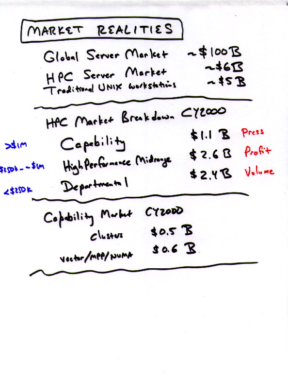
I think that $100B overstates the global server market somewhat, but this comparison does show the correct order of magnitude of the HPC market as a fraction of the overall server revenue opportunity. "Supercomputers" (in the traditional sense) make up less than 10% of the HPC server revenue, and less than 1% of the overall server revenue. Even this tiny fraction is further subdivided into vector systems, MPP systems, NUMA systems, and pseudo-vector systems.
Historically, supercomputer vendors have invested $200M to $400M in the development of new systems, and these numbers make it clear that such approaches cannot possibly break even. Assuming a system captures 50% of its segment (e.g., vector supercomputers), the total revenue over a three-year product life would be only about $300M. This can only justify a development budget in the $30M range -- far less than is required for even a derivative system design.

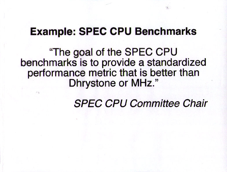
I bring in this quote not to beat up on SPEC, but to point out that the SPEC CPU subcommittee has not historically done the sort of research necessary to validate that the SPEC benchmarks are quantitatively representative of commercially important application codes. The SPEC CPU benchmarks are indeed much better figures of merit than MHz or Dhrystone MIPS, and have proven to be quite useful to both buyers and sellers of computer systems. Unfortunately, many have assumed that these benchmarks are also useful to designers of systems, and the data presented here shows that this assumption can lead designers in several wrong directions.

Another benchmark of interest is the LINPACK HPC benchmark. This (rather confusing) slide shows all of the available systems where I had application performance data and LINPACK data. In each case, the application performance was normalized to that of the 195 MHz SGI Origin2000 and used as the "y" value, and the LINPACK 1000 (aka LINPACK TPP) performance was also normalized to that of the 195 MHz SGI Origin2000.
The correlation is clearly approximately zero (the calculated value is 0.015), and the best-fit curve has a slope of 0.1 and a y-intercept of 0.9.
The bottom line is that LINPACK 1000 is useless for predicting the relative performance of these applications as a whole, though it is useful for a few of these codes individually (e.g., Abaqus/STD).
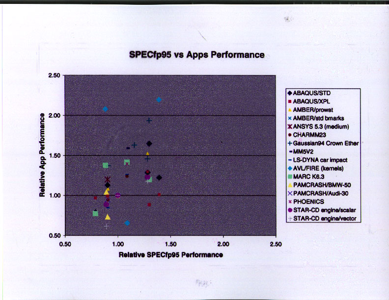
For this slide, I did the same analysis, except that I used SPECfp95 as the benchmark. It is important to note that these data points are for servers, and it is important to use the correct SPECfp95 benchmark -- the one measured on the server in question, not the best available SPECfp95 number for the same microprocessor (which is typically obtained on a workstation or a small, low-latency server). In this case, the correlation coefficient is about 0.39, the slope is approximately 1.0 and the y-intercept is approximately zero. The correlation is real, but quite "fuzzy".
Although I did not include the slide here, I did the same analysis using STREAM as the benchmark. As with LINPACK 1000, the correlation was very poor (correlation coefficient = 0.10). A harmonic combination of LINPACK 1000 and STREAM was able to do about as well as SPECfp95 (correlation coefficient = 0.36), but this required an "a posteriori" weighting of the two benchmarks to get good results. Nonetheless, this approach has some appeal, since running LINPACK 1000 and STREAM is immensely easier than running SPECfp95, and it makes sense for us to continue evaluating such an approach (especially since SPEC CPU2000 has become such a gargantuan benchmark, running for half a day or more on many current systems).
This is just a reminder that the work presented here was originally done by me and Ed Rothberg, while we were employed by Silicon Graphics, Inc. (now SGI). SGI's Chief Technology Officer (then Forrest Baskett, now retired from SGI) approved the release and publication of this work in August 1999, provided that the names of the applications were not disclosed. (Most of the licenses that SGI had with these software vendors prohibited the unilateral publication of benchmark results, and this data set does include performance-related information.)
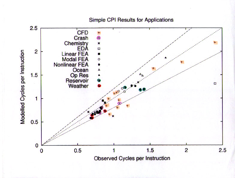
This slide shows the reconstruction of execution time (in cycles per instruction) based on twelve of the performance counters and a simple fixed-cost model for each of those twelve events. The cost for each event was guesstimated "a priori" based on my experience with the system under test, and not subsequently tuned.
The model included a CPI_0 component, calculated as MAX(LD+ST,FP,INT,BRANCH). This is equivalent to the assumption that these instruction types were fully overlapped by the out-of-order capability of the R10000 processor. The "core" component of the model also included a mispredicted branch penalty. The rest of the model consisted of memory subsystem components: Dcache miss, Icache miss, L2 data miss, L2 instruction miss, TLB miss, L1 cache writeback, L2 cache writeback.
Overall, this simple model was able to reproduce the actual CPI to within 20% for almost all cases. This is a fairly impressive result given that the model is based entirely on static estimates of costs and consists of 15 lines of "awk" (excluding the regular expressions that extract the performance counter data from the input files).

OK, we have finally gotten to real data!
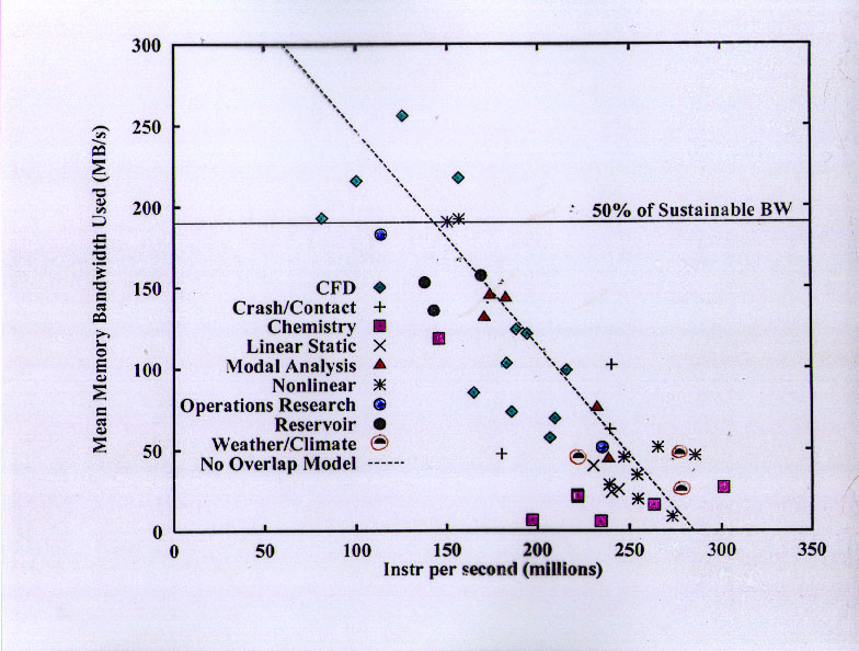
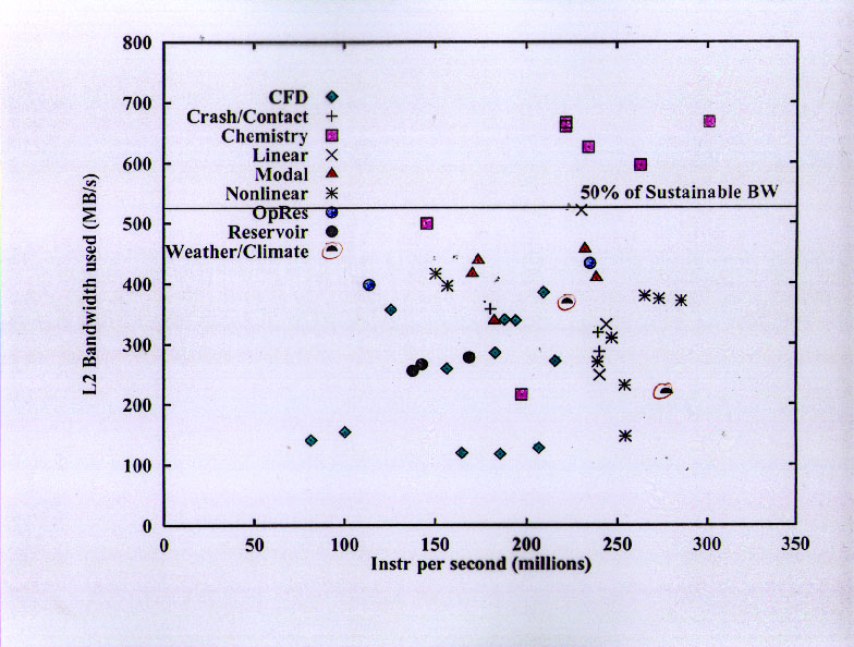
This slide shows the sustained instruction graduation rate on the x-axis and the average memory bandwidth utilization on the y-axis. The average memory bandwidth utilization is based on the total amount of memory transferred between the L2 and memory during the execution of the program, including data items not explicitly requested by the program (e.g., write allocate traffic and portions of cache lines that were not subsequently read).
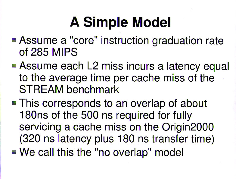
The dashed line is the "no overlap" model discussed on the previous slide, and the correspondence is quite good. The bottom line is that computations are not well overlapped with memory accesses, and memory accesses are slightly overlapped with each other. Part of this is due to the details of the SGI Origin2000 bus architecture, but part is due to the fundamental difficulty of tolerating cache misses that require many tens of processor cycles to satisfy. (On this machine, an L2 miss required 65 cycles before the data was available for use -- most modern machines have significantly higher values, and the trend is strongly upward.)
A very important message to be obtained from this slide is that lots of these applications used only a small amount of memory bandwidth. Almost half of them used only 50 MB/s or less -- about 1/8 of the maximum sustainable bandwidth of the Origin2000 memory bus, which delivers about 2 Bytes per processor cycle, or about 1 Byte per peak FLOPS.
Only a handful of applications would have used the full bandwidth of the processor if they had been able to run "infinite L2" speed, and almost all of these applications were in Computational Fluid Dynamics. There is one nonlinear FEA code that would probably use that much bandwidth, too, but comparison with the other codes leads one to believe that it is just badly written for cache-based systems. The final code in this regime is an optimization code running the Simplex algorithm for nondifferentiable optimization. It is strongly latency dominated.
The next group of codes includes the Petroleum Reservoir models and the Automotive Noise/Vibration/Harshness codes (eigenvalue solvers for FEA models). These would use up to about 1.5 Bytes/cycle if there were no memory stalls.
Next comes a group of CFD codes. Unlike the highest-bandwidth codes (many of which came from vector supercomputer environments), these CFD codes were developed in a "desktop" environment.
Finally, we see a large group of codes that run quite well, using minimal bandwidth. This group includes almost all the linear and nonlinear FEA codes (including the crash codes), the weather and climate models, the computational chemistry codes, one modal analysis code, one operations research code (solving a mixed linear programming problem). It is important to emphasize that none of these codes were running "toy" cache-containable problems. They exhibit excellent cache re-use because they have been tuned by experts to use hierarchical memories effectively, and because the basic algorithms of interest tend to be computationally "dense" (i.e., they require many arithmetic operations per update of each data value).

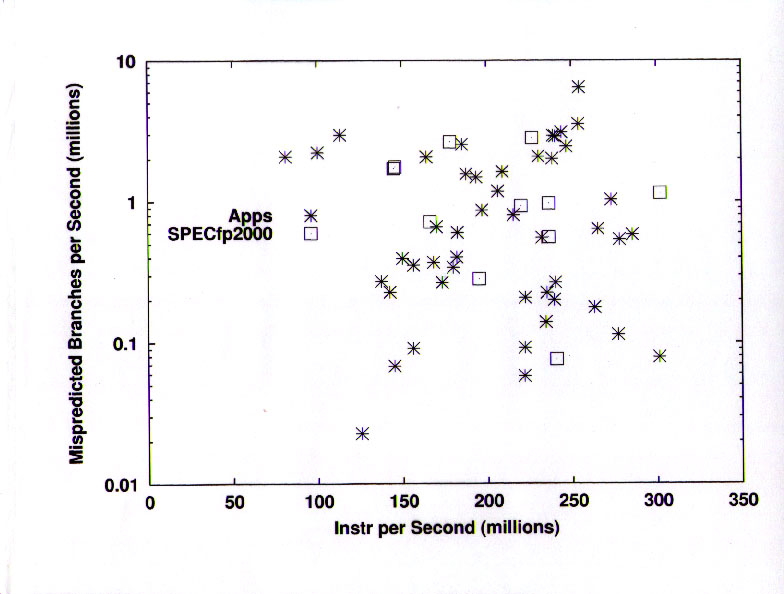
Here I have grouped the applications together and compared with the SPEC CFP2000 benchmarks.
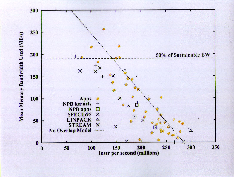
Here is the comparison with a broader benchmark set.
Although the benchmarks clearly cover the same overall range as the applications, the benchmarks do not have good coverage of the "cache-friendly" subset of the applications.
Here we see the L2 bandwidth utilization of the application areas. Note that the highest L2 bandwidth utilization (just over 50% of the maximum sustainable L2 bandwidth) is in the set of applications with the lowest main memory bandwidth demand (computational chemistry).

The SPEC CFP2000 benchmarks are clearly not representing what is going on in the applications here. Most have very low bandwidth utilization, and only one of the codes exceeds 40% utilization. One of the reasons for this is that none of the SPEC CFP2000 codes are explicitly "blocked" for cache re-use. Another reason is that the SPEC CFP2000 codes tend to be algorithmically very simple, while the commercially important applications are doing a lot more complex "work" on each data element.
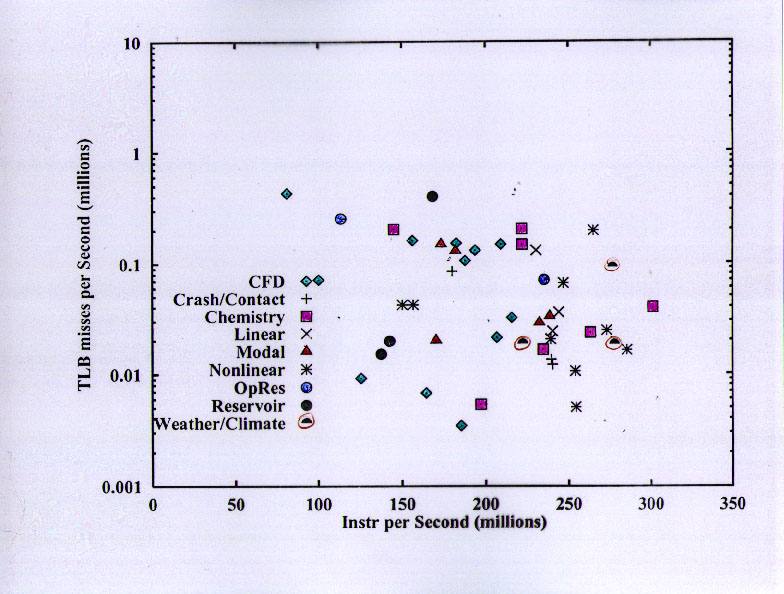
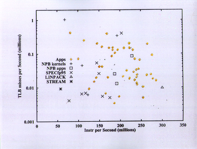
The Translation Lookaside Buffer (TLB) miss rates of the benchmarks are mostly pretty low compared to the applications.
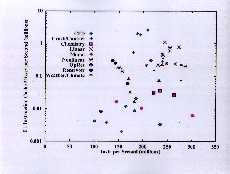

The Icache miss rates of the CFP2000 benchmarks are mostly very much lower than those of the applications.
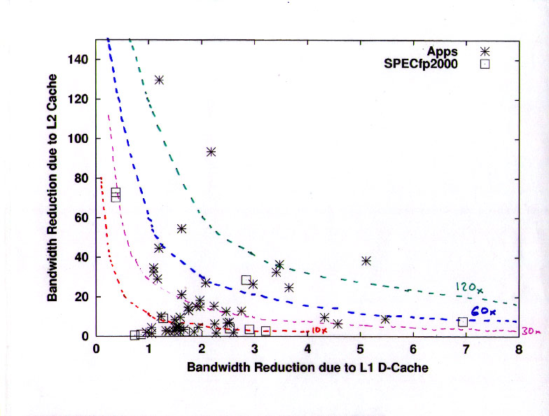
This confusing slide tries to convey the cache re-use of the L1 and L2 caches for data items. In each case the "re-use" factor is defined as the ratio of the data transferred "inbound" (toward + from the CPU) to the data transferred "outbound" (toward + from the next higher level of the memory hierarchy).
The important feature here is that most of the applications have significant L2 reuse factors. A large fraction of the applications have L2 reuse factors in the range of 10 to 40, while only one of the SPEC CFP2000 benchmarks shows this behavior.
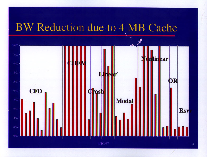
Here is another view of the L2 reuse parameter, by application area. The y-axis is truncated at 20 in this slide, though most of the chemistry applications have re-use factors of about 100.
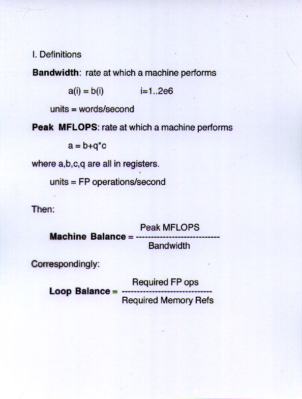
Now I am going to talk about the "balance" between bandwidth and compute capability, using these definitions.
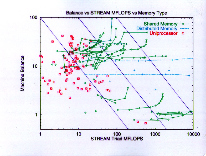
This is fairly old data, but definitely shows four groups

Here are some names to attach to the same data.
Historically, machines with balance significantly greater than about 20 have had little market success in scientific and technical accounts, except in select application segments (e.g., computational chemistry or seismic data processing) which tend to be extremely cache-friendly.
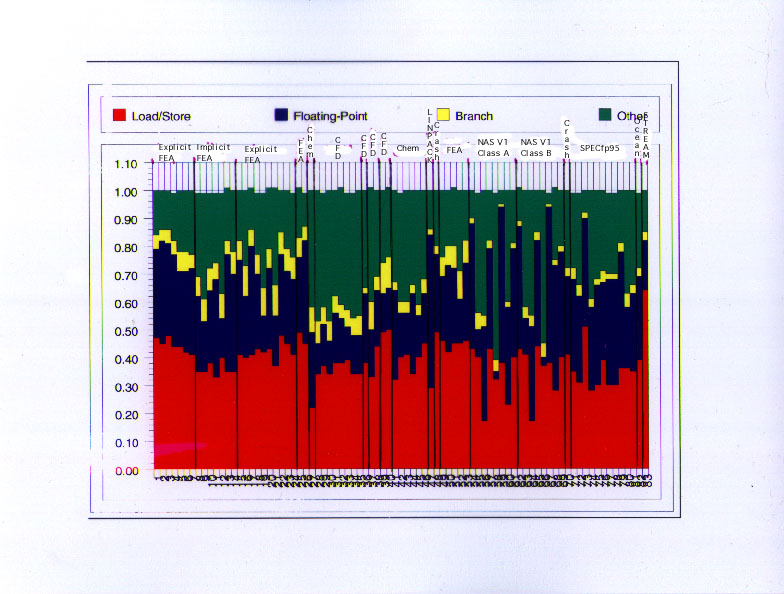
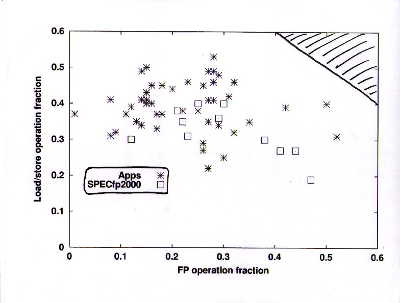
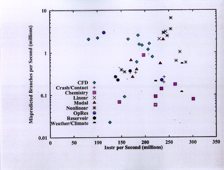
On to a new topic --- dynamic distribution of instruction types. The basic information from this chart is that different applications have dramatically different instruction distributions, and that most of the applications have a lot more load/store instructions than floating-point instructions.
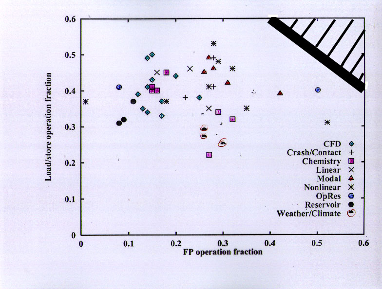
Some detail on the percentage of load/store instructions vs the percentage of floating-point instructions for the applications. Although the ratio varies considerably, almost all of the applications have significantly more than one load/store per FP instruction (note that floating-point multiply-add is counted as one instruction on this machine), and many of the applications are at a ratio of about 2.
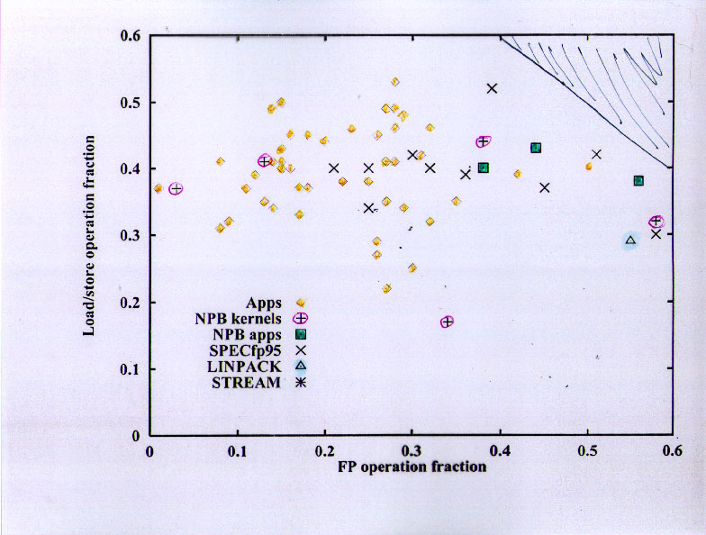
The benchmarks have a lot more floating-point than the applications, with generally similar load/store fractions. Some benchmarks approach two FP per load/store, while most are at about a 1:1 ratio.