This page does not represent the most current semester of this course; it is present merely as an archive.
1 Overview
In this assignment you’ll draw 2D shapes by filling in individual pixels.
Optional part point values and examples will be added soon.
1.1 Logistics
You need to write every method you submit yourself. You cannot use other people’s code or find the method in an existing library. For example, you should not use Java’s Graphics class, PIL’s ImageDraw module, the CImg draw_* methods, the Bitmap Draw* methods, etc.
You are welcome to seek conceptual help from any source, but cite it if you get it from something other than a TA, the instructor, or class-assigned readings. You may only get coding help from the instructor or TAs.
Half of the points are for completing the required portions. You may add as many points as you wish on optional portions. Points in excess of 100% will carry over to other homework assignments.
1.2 Structure and File Format
The same as HW0: your program will read a file from the command line and create a PNG file. The basic structure of the input file (lines with keywords and arguments, skipping unknown keywords, etc) remain unchanged.
2 Required
The required part is worth 50%
png
same as HW0
xyc, xyrgb
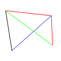
For this homework, when you see a vertex description line (xyc, xyrgb, or the optional xyrgba) you don’t draw it; you store it in an ordered list. Most other commands will refer to earlier vertices in a one-indexed way: 1 is the first vertex listed, −1 the most recent one listed. So, for example, in the following input file
the indices on the two trig lines refer to the vertex lines of the corresponding color.
Vertex indices will always refer to vertices earlier in the file. Vertex coordinates (\(x\) and \(y\)) may be decimal numbers. Colors will still be integers. You no longer need to support xy; all coordinates will have colors specified in this assignment.
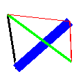
linec \(i_1\)\(i_2\)hexcolorcode
Draw an 8-connected line of the given color using the DDA algorithm between the two vertices given. Ignore the colors of the vertices.
If the line extends farther in \(x\) than in \(y\), fill the pixel with \(y\) of \(⌊liney + 0.5⌋\) for each integer \(x\) between the \(x\) coordinates of the two vertices. If it extends farther in \(y\) than in \(x\), fill the pixel with \(x\) of \(⌊linex + 0.5⌋\) for each \(y\) between the \(y\) coordinates of the two vertices. In the case where you start or end with an integer endpoint, include the smaller value but not the larger. For example, if stepping between 20 to 10, include 10 but not 20.
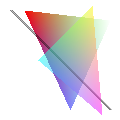
trig \(i_1\)\(i_2\)\(i_3\)
Fill a triangle between the given vertices, linearly interpolating the vertex colors as you go. Use a DDA-based scanline algorithm: DDA step in \(y\) along the edges, then loop in \(x\) between these points.
Fill a vertex if its coordinates are inside the triangle, (e.g., pixel \((3, 4)\) is inside \((2.9, 4)\), \((3.1, 4.1)\), \((3.1, 3.9)\)) on the left (small \(x\)) edge of the triangle, or on a perfectly horizontal top (small \(y\)) edge. Do not fill it otherwise.
This coloring style is called Gouraud shading, hence the g in the keyword.
3 Optional
3.1 Colors
lineg \(i_1\)\(i_2\) (5%)
Linearly interpolates colors on lines
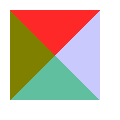
tric \(i_1\)\(i_2\)\(i_3\)hexcolorcode (5%)
Fills a triangle as trig but uses the specified flat color, not linearly-iterpolated color
xyrgba or lineca/trica (10%)
Accept points xycrgba with a 4th color being an alpha (opacity) channel, and use that alpha in Gouraud shading (lineg and trig).
And/or, add lineca and trica that act like linec and tric but take an extra 2 hex digits in the color code, which are alpha (opacity). So #ff0000ff is opaque red, #0000ff07 is mostly transparent blue, etc.
Use the over operator discussed on Wikipedia: \(C_{o}={\frac {\alpha_{a}}{\alpha_{o}}}C_{a}+\left(1-{\frac {\alpha _{a}}{\alpha _{o}}}\right)C_{b}\).
Fill the given n-vertex polygon using the even-odd rule, as described in the SVG Spec.
Usually this is best done by going one scanline at a time, finding all of the edges that cross it, and then filling between pairs. Don’t forget to count vertexes that fall exactly on a scanline appropriately.
Fill the given n-vertex polygon using the non-zero rule, as described in the SVG Spec.
Usually this is best done by going one scanline at a time, finding all of the edges that cross it, and then filling between pairs. Don’t forget to count vertexes that fall exactly on a scanline appropriately.
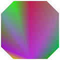
fann \(n\)\(i_1\)\(i_2\) … \(i_n\) (10%)
Goaraud fill a polygon between \(i_1\) and each adjacent pair of subsequent vertices (e.g., \(i_1\)\(i_2\)\(i_3\) and \(i_1\)\(i_3\)\(i_4\) and …).
stripn \(n\)\(i_1\)\(i_2\) … \(i_n\) (10%)
Goaraud fill a polygon between each three consecutive indices (e.g., \(i_1\)\(i_2\)\(i_3\) and \(i_2\)\(i_3\)\(i_4\) and …).
linewc \(i_1\)\(i_2\)\(w\)hexcolorcode (10%)
Draw a line as a rectangle with width \(w\) touching the two endpoints (line butt mode in the SVG spec).
Draw a cubic bezier curve of the given width. Usually this is done by turning the boundary of the curve into a polygon with a lot of vertices, adding two of the vertices at every step of De Caustlejau’s algorithm.
cubicg \(i_1\)\(i_2\)\(i_3\)\(i_4\) (10%)
Draw a cubic bezier curve interpolating the vertex colors as you go.
Draw a cubic bezier curve where the width is interpolated along the curve. Usually this is done by turning the boundary of the curve into a polygon with a lot of vertices, adding two of the vertices at every step of De Caustlejau’s algorithm.
Draw a uniform cubic B-spline with the given control points.
A B-spline is just a tool for defining Bezier curves. The B-Spline control points \(p_1\), \(p_2\), \(p_3\), \(p_4\) define the cubic Bezier control points \((p_1 + 4p_2 + p_3)\over 6\), \((2p_2 + p_3) \over 3\), \((p_2+2p_3) \over 3\), \((p_2 + 4p_3 + p_4) \over 6\).
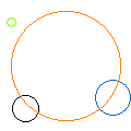
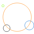
circle \(i_1\)radius (15%)
Draw the outline of a circle centered at the given vertex with the given radius. Use the color of the vertex. You may assume the center vertex has integer coordinates and the radius is an integer.
3.4 Antialiasing
aalinec \(i_1\)\(i_2\)hexcolorcode (10%)
Draw an anti-aliased line using the Wu algorithm. Use the over operator to compose transparent pixels.
aacircle \(i_1\)radius (10%)
Draw an anti-aliased circle using the Wu algorithm. Use the over operator to compose transparent pixels.
3.5 Other
Feel free to add your own elements to the input set. Submit an input file named additional_.txt where _ is replaced by some number for each additional element you add. The input file should include a line beginning description that describes the new element. Points will be added at instructor discretion.